This time I’ll focus on stellar classes and some of their most important (and unique) features to help navigate right to your choice. If you are reading this, I assume that you’ve probably looked through some other articles about stellar classes elsewhere (e.g. Wikipedia, Stellar classification) and deliberately search for more detailed info for your future world-to-be. This is exactly what I have in mind, presenting current article on stellar species and their natural habitat.
House of beasts
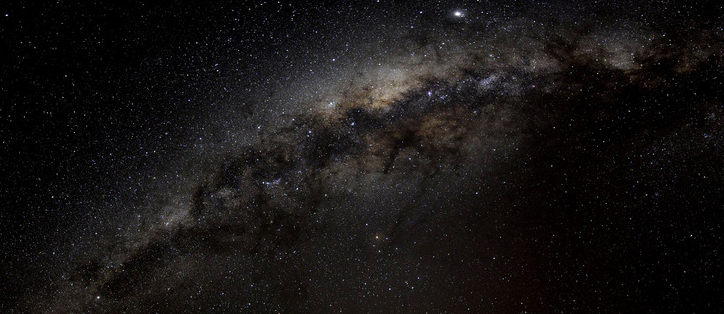
Our star is a member of a giant cosmic structure known as the Milky Way Galaxy, along with up to 400 billion other stellar folks. It is agreed that the Milky Way is a spiral galaxy, with observations suggesting that it is a barred spiral galaxy. Its stellar disk is approximately 100 000 light-years (30 kiloparsecs, 9*10^17 km) in diameter and is considered to be, on average, about 1 000 ly (0.3 kpc) thick.
The Milky Way is part of the Local Group of galaxies and is one of hundreds of billions galaxies in the observable universe. And that’s a lot of places to reside in, at least in fiction.
So, what is so special about our Galaxy? The answer is simple: we know it has life – us.
Not every galaxy in the universe is suitable for life (as we know it – sorry, I’ll stick with this again since I’m very interested in it being a member of one myself). So, if you are choosing a stellar home from a range of existing galaxies, take a good look at its specs. Galaxies can be distinguished by shapes, sizes, composition and stellar formation activity, and their relationships with neighbors. They are dynamic systems and very violent ones, to that. They live and they die, and they feed on their own kind.
Now, let’s look at the features of our stellar home and how is it suitable for life to exist.
It’s a spiral galaxy with relatively high chemical abundance of interstellar medium, active stellar formation regions and calm places far away from hazardous to life star forming regions.
Two huge bubbles that emit gamma rays have been found billowing from the center of the Milky Way galaxy, extending 25,000 light-years north and south from the galactic core. Gamma rays are the most energetic forms of light, and in space they tend to come from violent events such as supernovae or from extreme objects such as black holes and neutron stars.
These bubbles are made of hot, charged gas that’s releasing the same amount of energy as a hundred thousand exploding stars. Scientists are conducting more analyses to better understand how the structure was formed. One possibility includes a particle jet powered by matter falling toward the supermassive black hole at the galactic center. While there is no evidence the Milky Way’s black hole has such a jet today, it may have in the past. When galactic black holes are actively feeding, they tend to spew jets of particles traveling at nearly the speed of light. Astronomers have found such active galactic nuclei elsewhere in the universe, but have never before seen any convincing proof of this process happening in the Milky Way. The bubbles also may have formed as a result of gas outflows from a burst of star formation, perhaps the one that produced many massive star clusters in the Milky Way’s center several million years ago. If that’s the case, the giants could now be dying together, creating an outbreak of supernovae.
Update Jan 2013: observations tell the bubbles are star-power.
Update Sept 2013: around 2 million years ago, a bright moon-sized smudge was also visible in Earth’s southern sky.
Update August 2014: Despite extensive analysis, Fermi bubbles defy explanation. The mystery remains.
Galaxies are in motion and they crash into one another from every conceivable direction. It is believed that Andromeda and the Milky Way galaxies will collide in just a few billion years. During the collision our Sun and solar system may be stripped away from its present orbital radius and come to reside in Andromeda. If the two galaxies merge they will form an elliptical galaxy.

Galaxies exchange stars. In fact, some of the stars from the Sagittarius Dwarf Elliptical Galaxy (SDEG) may have been captured by the Milky Way billions of years ago (Chou, et al., 2009; Majewski et al., 2003). Moving in a roughly polar orbit around the Milky Way as close as 50,000 ly from its galactic center (Ibata et al., 1997), SDEG comes far too close to the Milky Way for the dwarf to remain intact from the resulting gravitational tides. Here is a dramatic display of galactic cannibalism. Although it may have begun as a ball of stars before falling towards the Milky Way, SDEG is 10,000 times smaller in mass than the Milky Way, so it is getting stretched out, torn apart and gobbled up by our Galaxy. The Canis Major Dwarf Galaxy (CMDG) is even closer (Martin et al., 2004). SDEG and CMDG are both older galaxies and the Milky Way likely stripped millions of stars from them (Chou, et al., 2009; Martin,et al., 2004; Majewski et al., 2003).
Our Galaxy hosts more than a dozen known stellar streams, the remnants of satellite galaxies that were gravitationally torn apart and consumed. Most of the other streams loop around the plane of our disk-shaped galaxy, like octopus tentacles grasping a dinner plate.
The Milky Way has 14 known dwarf galaxies orbiting it, and recent observations have also led astronomers to believe the largest globular cluster in the Milky Way, Omega Centauri, is in fact the core of a dwarf galaxy with a black hole in its center, which was at some time absorbed by the Milky Way.
If colliding, merging, and interacting galaxies and their stars and solar systems harbored life, then not just stars, but living organisms would have also been transferred between galaxies. Therefore, even if life had been fashioned only once, in some ancient galaxy which predates our own, the descendants of this life form could have easily journeyed from planet to planet, from solar system to solar system, and from galaxy to galaxy.
A living planet with an atmosphere, orbiting within the habitable zone of a sun-like star, will be subjected to that star’s solar winds. In the case of Earth, the powerful magnetic field protects the planet from these winds. These winds will periodically increase significantly in strength and eject air-born microbes into space and distribute them not just to neighboring planets, but outside the solar system where they may come to contaminate collections of Oort Cloud stellar objects and passing comets. After hundreds of millions of years survivors may fall upon a planet orbiting a distant star.
However, this does not mean that all this free floating molecular material would have achieved life. It needs the right address and the right time of delivery. Nevertheless, given even the odds of 1 in a trillion, it can be predicted that life could have arisen in multiple galaxies through chance combinations of the necessary ingredients in the nebular clouds.
So, the question is which galaxies are best suited for life formation and evolution?
We may consider galaxies as composed of some “building blocks” whose scale and importance varies from galaxy to galaxy. These include a nucleus, bulge, lens, bar, spheroidal component, disk (with arms, rings, etc), and an unseen halo which is significant for the mass distribution and dynamics. The order revealed by existing classification systems tells us that these are not really independent; disk/bulge correlates overall with arm morphology, for example. These relations hold clues to both the formation and evolution of galaxies, and their suitability for life.
Looking at these classification systems, I can name at least four galactic factors that are vital for our objective: stellar population, chemical abundances in the interstellar medium, star formation history along with integrated stellar spectrum and location of potential life-bearing system in the galaxy.
A spiral galaxy like the Milky Way contains stars, stellar remnants and a diffuse interstellar medium (ISM) of gas and dust. This medium has been chemically enriched by trace amounts of heavier elements that were ejected from stars as they passed beyond the end of their main sequence lifetime. Higher density regions of the interstellar medium form clouds, or diffuse nebulae, where star formation takes place. In irregular galaxies, they may be found throughout the galaxy, but in spirals they are most abundant within the spiral arms. A large spiral galaxy may contain thousands of H II regions.
Together with irregulars, spiral galaxies make up approximately 60% of galaxies in the local Universe. They are mostly found in low-density regions and are rare in the centers of galaxy clusters.
In contrast to spirals, an elliptical galaxy loses the cold component of its interstellar medium within roughly a billion years, which hinders the galaxy from forming diffuse nebulae except through mergers with other galaxies. Gas is the raw building material for stars and the more gas a galaxy contains, the more stars are born.
Most elliptical galaxies are composed of older, low-mass stars, with a sparse interstellar medium. Star formation is minimal or has finished after the initial burst, leaving them to shine with only their aging stars. In general, they appear yellow-red, which is in contrast to the distinct blue tinge of a typical spiral galaxy, a color emanating largely from the young, hot stars in its spiral arms.
Elliptical galaxies are believed to make up approximately 10–15% of galaxies in the local Universe but are not the dominant type of galaxy in the universe overall. They are preferentially found close to the centers of galaxy clusters and are less common in the early Universe.
Despite the prominence of large elliptical and spiral galaxies, most galaxies in the universe appear to be dwarf galaxies. These galaxies are relatively small when compared with other galactic formations, being about one hundredth the size of the Milky Way, containing only a few billion stars. Star formation in dwarf galaxies appears to be complex, with many systems exhibiting multiple episodes of star formation.
Take, for example, the Magellanic Clouds (Large Magellanic Cloud and Small Magellanic Cloud). These dwarfs are members of our Local Group and are orbiting our Galaxy. While both are often considered an irregular type (the NASA Extragalactic Database lists the Hubble sequence type as Irr/SB(s)m), they contain very prominent bars in their centers, suggesting that they may have previously been barred spiral galaxies. Aside from their different structure and lower mass, they differ from our Galaxy in two major ways. First, they are gas-rich; a higher fraction of their mass is hydrogen and helium compared to the Milky Way. They are also more metal-poor than the Milky Way; the youngest stars in the LMC and SMC have a metallicity of 0.5 and 0.25 times solar, respectively. Both are noted for their nebulae and young stellar populations, but as in our own Galaxy their stars range from the very young to the very old, indicating a long stellar formation history.
There are, of course, other morphologies, like ring or lenticular galaxies, for example.
If you have further interest in galaxies, I suggest reading “Galaxy Morphology and Classification” by Sidney van den Bergh.
Stellar populations and their habitat
Stars are the building blocks of galaxies. They are formed continuously in some galaxies, and only in bursts in others. The term stellar population is used to refer to a single generation of stars characterized by a common age and chemical composition. A galaxy can be composed of a large number of individual populations. Stellar populations are not discrete in their properties, but rather have a continuum of characteristics that reflect the changes in star formation with time. Stellar populations are tracers of events in galaxy’s past and formation.
A young (less than 100 Myr) population contains massive stars. These are hot and generate much blue light. An old (more than 3 Gyr) population contains no massive, hot stars, only cool low-mass stars on the main sequence and red giants. It is therefore yellow-red in color. A very young population (less than 10 Myr) produces much ionizing radiation, which creates H II regions in the surrounding gas, whose spectra contain strong emission lines. The dominant emission line of hydrogen gives such regions a characteristic pinkish tint in color images. Thus, the integrated color of a stellar population is a function of its age, and this relation can be used to age-date populations in distant galaxies.
The Hertzsprung-Russell (HR) diagram is the basic tool for analyzing the temperature distributions of evolving stellar systems.

In the HR diagram temperature (increasing to the left) is plotted against instrinsic stellar brightness or luminosity (increasing upward). Most stars fall on the main sequence (MS), which runs diagonally across the HRD. More massive stars on the MS are brighter and hotter, hence bluer. MS stars maintain themselves by burning hydrogen in their cores. But when they run out of H fuel, they evolve off the MS (to the right, or toward lower temperatures, in the diagram). More massive stars evolve faster. A single generation will have stars with a large range in mass, which means that its HR diagram will change as the more massive stars evolve.
You may also enjoy playing with the following HR Diagram Explorer.
There are basically three stellar populations in our Galaxy, corresponding to the three distinct dynamical components to the Galaxy; the disk population, the bulge population and the halo population. The disk population inhabits the rotating, flattened region of our Galaxy. The bulge population is restricted to the rounded, central region of the Galaxy, also rotating. And the halo population inhabits the far outer regions of the Galaxy, on long ellipisodal orbits that takes it into the disk and bulge.
The three components not only have distinct kinematic properties, but the types of objects in them also varied. The disk contains all the gas and young stars, although old stars are also found there. The bulge is dominated by old stars and a violent core. The halo contains very old stars and globular clusters. The reason for this separation of stellar types is a clue to how the Galaxy formed.
Disk and bulge stars tend to be rich in heavy elements (above helium on the periodic table). Halo stars tend to be very poor in heavy elements. Changes in the chemical composition of a star are due to the initial chemical composition of the gas cloud that it was born from. This heavy elements are mostly produced by supernova explosions, gas clouds become enriched by the ejecta of supernova. The larger the number of supernova near a cloud, the richer in heavy elements it will become. As time passes, each of the gas clouds in the Galaxy will increase in the abundance of elements such as carbon, iron, etc. So the more recent a star has been formed, the richer in heavy elements it is. This is a form of dating system for stars and we deduce that halo stars are the oldest stars in the Galaxy since they have the lowest chemical abundances. The disk stars are the youngest since they are the most metal rich.

Thin disk (Population I)
The thin disk of the Milky Way has sustained ongoing star formation for ~10^10 years. Consequently it contains stars with a wide range of ages, and the thin disk may be divided into a series of sub-populations of increasing age.
The spiral-arm population is the youngest in the disk; it appears to trace the spiral pattern of the Milky Way. This population is concentrated very close to the disk plane, with a scale height of ~100 pc. Representative objects include H I and molecular clouds, H II regions, protostars, stars of types O & B, supergiants and classical cepheids. The metallicity of this population is somewhat higher than that of the Sun. As the young stars age, they drift out of the spiral pattern.
The disk population is more smoothly distributed and does not seem to trace the spiral structure. This population may be further subdivided into young, intermediate, and older categories, with ages of ~1, ~5, and ~10 billion years, respectively. The characteristic scale-height of this population increases with age, ranging from ~200 to ~700 pc, while the metallicity declines to perhaps ~20% of the solar value. Representative objects include stars of type A and later, planetary nebulae, and white dwarfs. Our Sun is a member of this group.
Population I stars have regular elliptical orbits around the galactic centre, with a low relative velocity. The high metallicity of Population I stars makes them more likely to possess planetary systems than the other two populations, since planets, particularly terrestrial planets, are thought to be formed by the accretion of metals.
Stellar halo (Population II)
The stellar halo of the Milky Way includes the system of globular clusters, metal-poor high-velocity stars in the solar neighborhood, and metal-rich dwarf stars seen toward the galactic center. While star formation in the outer halo largely ceased more than 10^10 years ago, the situation in the inner kpc of the galaxy is not so clear.
Globular clusters are the classic tracers of the galactic halo. The metal-poor clusters have a nearly-spherical distribution extending to many times the Sun’s distance from the galactic center, while the metal-rich clusters are concentrated towards the center of the galaxy and may have a more flattened distribution.
Metal-poor subdwarfs in the solar neighborhood have large velocities with respect to the Sun and other disk stars. These stars are on highly eccentric orbits about the galactic center; the net rotation of this population is amounts to less than ~40 km/sec, while their random motions are quite large. The metallicity of these stars ranges from ~0.1 to ~10% of solar.
Metal-rich subdwarfs in the central bulge of the galaxy span a wide range of metallicity, from ~0.1 to > 100% of solar. The inner kpc of the bulge also appears to contain stars of type A, implying that some star formation has occurred rather recently.
Thick disk (Intermediate Population II)
Intermediate Population II stars are common in the bulge near the center of our Galaxy; star-counts suggest that this intermediate population is distributed in a thickened disk with a scale height of ~1 to 1.5 kpc. This population accounts for only ~1% of the stars in the vicinity of the sun but dominates the high-altitude tail of the thin disk population at z > 1 kpc.
Kinematic studies imply that the thick disk rotates with a velocity of ~180 km/s, compared to the less than 40 km/s rotation of the metal-poor subdwarfs. This would indicate that the thick disk is more closely associated with the thin disk population, which rotates at ~220 km/s. Metallicity measurements also support the idea that the thick disk is distinct from the stellar halo; the characteristic metal abundance of thick disk stars is ~25% of solar, while the stellar halo is significantly more metal-poor in the solar neighborhood.
If you decide to go further into gory details of galactic kinematics, you should check Astrophysical Formulae, Volume II: Space, Time, Matter and Cosmology, K. R. Lang, 3rd ed., pp 42-47.
Also, you could check this site or this one for rotation curve of the Galaxy.
Taxonomy of dragons
The vast majority of stars are main sequence stars – these are star like the Sun that are burning hydrogen into helium to produce their energy. Most stars spend 90% of their life as main sequence stars.
The spectral types and subclasses represent a temperature sequence, from hotter O stars to cooler M stars, and from hotter subclass 0 to cooler subclass 9. The temperature defines the star’s “color” and surface brightness. The luminosity class designation describes the size (gravitational acceleration in photosphere) of a star from the atmospheric pressure. For larger stars of a given spectral type, the surface gravity decreases relative to what it was on the main sequence, and this decreases the equivalent widths of the absorption lines.
There are several classes of luminosity: 0 – Hypergiants (extremely luminous), Ia – Bright Supergiant Stars (large and luminous), Ib – Supergiants (less luminous than Ia*), II – Bright Giants, III – Giants, IV – Subgiants, V – Main Sequence, sd – Sub-Dwarfs, D -White Dwarfs. *Classes can be categorized like: Ia, Ib, Ic, IIa, IIb, IIc, and so on (sub-a being brighter that sub-b).

Stars are clearly distinguished according their spectra: O type stars are the brightest and the live the shortest; B type stars are blue white and also burn bright, but not as bright as the O type; A type stars are less bright, a little larger than our Sun, but still a lot hotter; F – Brighter than our Sun and a little hotter; G – Our Sun is a G type star; K – dimmer that our Sun, with longer lifespan because temperature is lower; M – the dimmest stars, will burn for a long time. Each spectral type is divided into 10 subclasses, A0, A1, A2, …A9 etc.
Spectrum features for each class according to element radiation lines must be considered. O stars – strong HeII (He+) lines, in absorption or emission; strong UV continuum; weak HeI, prominent H lines; SiIV, OIII, NIII, CIII. B stars – strong HeI in absorption; HII absent; H lines stronger; MgII, SiII. A stars – H lines at max in A0; HeI & HeII absent; FeII, SiII, MgII at max; some CaII; weak neutral metals. F stars – H lines weaker; CaII H&K stronger; neutral metals stronger. G stars – CaII lines dominate; H very weak; FeI, MnI, CaI become stronger; CH G-band strong. K stars – neutral metals strong; TiO bands appear. M stars – neutral metals and molecules (CH, TiO, etc.)

The complete spectral type (e.g., F5V) nearly uniquely places a star in the HR diagram. Classification schemes assume solar abundances and slight changes are needed for metal-poor stars.
Many stars have peculiar features, their spectral types are coded with additional designations.
To explore each stellar class in greater detail, you can look through this data.
Luminosity and temperature are not the only important properties of stars and I will be returning to this theme some time later, in context of habitable worlds.
P.S. I’ve avoided the term Galactic Habitable Zone on purpose for several reasons. One of them being a thought that in galaxies similar to our own, stars such as the Sun can migrate great distances, thus challenging the notion that parts of these galaxies are more conducive to supporting life than other areas. It’s the same as saying some parts of a well built road are better for traffic than others. Accidents happen, just not with everyone during the ride. Also, some circumstances may result in suitable planets outside the defined “habitable zone”. And there’s always the probability of life as we don’t know it.