From Stars to Planets: The Loners

Brown dwarf glows feebly in the dark depths of space. Artwork by David Aguilar, Harvard-Smithsonian CFA

The word planet means “wanderer”; the Greeks called them planētēs aster, “wandering stars”. Indeed planets travel on their orbits, wandering around their stars for millions and billions of years. Stars move along their paths in galaxies, wandering, until the end of their time. Some objects, however, do not follow this familiar pattern. These objects include planets, brown dwarfs, stars, and even black holes, bringing up the most challenging setting for a science fiction story.

Shadowy neighbors

Our Galaxy alone is full of unusual stuff. Objects known as brown dwarfs were only a theoretical concept until they were first discovered in 1995. It is now argued that there might be as many brown dwarfs as there are stars, and our closest neighbor might turn out to be an ultracool brown dwarf rather than Proxima Centauri.

Brown dwarf glows feebly in the dark depths of space. Artwork by David Aguilar, Harvard-Smithsonian CFA

These objects fall somewhere between the smallest stars and the largest planets on the heavenly spectrum, and have masses that range between twice the mass of Jupiter and the lower mass limit for nuclear reactions (0.08 solar masses). They are thought to form the same way low-mass stars do – from a collapsing cloud of gas and dust. However, as the cloud collapses, it does not form an object which is dense enough at its core to trigger and maintain hydrogen-burning nuclear fusion reactions. Their spectral characteristics are different to those of very cool stars, showing an absorption line of the short-lived element lithium. Furthermore, they have fully convective surfaces and interiors, with no chemical differentiation by depth. In young brown dwarfs, when combined with rapid rotation, their turbulent interior motion can lead to a tangled magnetic field that can heat their upper atmospheres, or coronas, to a few million degrees Celsius. Even if not fusion powered, these mysterious objects are also known to have flares.

The nuclear fusion is what fuels a star and causes it to shine, but brown dwarfs are very cool and dim compared to stars. The coolest brown dwarf yet discovered is about as hot as boiling water, with a temperature of less than 100 degrees Celsius (~ 370 K).

Update September 7th 2013: A new study shows that some brown dwarf stars may be as cool as room temperature.

Dwarf comparison: from stars to planets

The trouble with brown dwarfs is that they are hard to find. An isolated (not in a multiple system) brown dwarf is typically visible only at ages < 1 Gyr because of the rapidly fading luminosity. The lighter brown dwarfs are more sensitive to this effect. Young brown dwarfs are visible at relatively large distances but evolve rapidly, making it difficult to catch them when they are in their earliest stages of formation. Old brown dwarfs will only be visible if they are nearby. So we have more chance of discovering brown dwarfs that have just recently formed.

Dumping more mass on a brown dwarf doesn’t make it bigger, it just makes it denser. A 70-Jupiter-mass and 20-Jupiter-mass brown dwarf are both about the size of Jupiter.

From up close, a young brown dwarf would look like a low-mass star, but an old brown dwarf would look more like Jupiter.

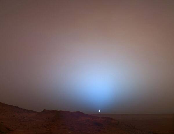
Brown dwarfs aren’t brown, they would look red to the naked eye.

Brown dwarfs radiate most of their energy in infrared light.

Some brown dwarfs spin so fast that they complete one rotation in less than an hour.

Brown dwarfs have hydrogen cores.

The average density of a brown dwarf is about 70 grams per cubic centimeter, which is 5 times the density at the center of the Earth.

Robert Naeye, Astronomy magazine, August 1999, p. 36-42

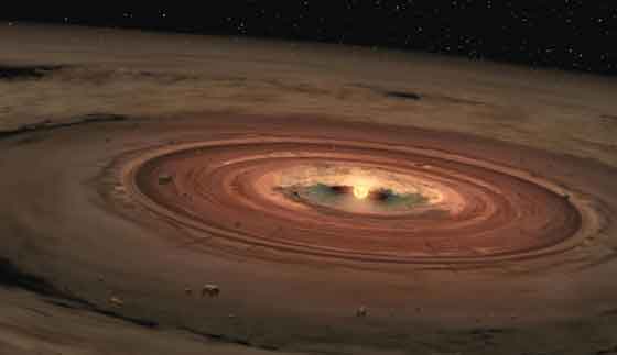
Brown dwarfs have also been discovered embedded in large clouds of gas and dust. Accretion discs were detected around some of these failed stars, even around those as small as 10 Jupiter masses. Astronomers discovered that some disks contain dust particles that have crystallized and are sticking together in what may be the early phases of planet assembling. A relatively large and many small grains of mineral called olivine was found; another sign of dust gathering up into planets is the flattening of brown dwarfs’ disks. But such systems will be tiny compared to our own Solar System.

Brown dwarfs emit faint visible light, but are cool enough to retain a somewhat Jupiter-consistent atmosphere. For example, Gliese 229B, discovered in 1995. Its luminosity is about one tenth of the faintest star and its spectrum has large amounts of methane and water vapor. Methane could not exist if the surface temperature were above 1200K. Astronomers consider its temperature to be about 950K (compared to Jupiter’s 130K), its mass to be between 0.02 and 0.05 of solar, and the age of the binary system to be between 2 and 4 billion years. It has a smoggy haze layer deep in its atmosphere, essentially making it, much fainter in visible light than it would otherwise be. It is possible that ultraviolet light from its companion star changes its atmospheric properties from those of an isolated brown dwarf. Theory now also suggests that young brown dwarfs are hot enough (with temperatures as high as 2000 Kelvin) to have clouds of iron and silicates. These clouds “rain out” as the brown dwarf cools and becomes dimmer. But this raining out causes a temporary brightening as obscuring clouds are cleared from the atmosphere. Considering the age and the temperature of Gliese 229b, its atmosphere should be clear of clouds, leaving it a featureless ball glowing a dull red, like a coal, from internal heat. Any moons that might had formed too close to the brown dwarf would have been torn apart by tidal forces long ago. Surviving moons, if they exist, may be heated enough by tidal forces for methane or nitrogen geysers to form.

This paper describes a collection of evolutionary models for brown dwarfs and very-low-mass stars for different atmospheric metallicities, with and without clouds.

Children of the Demon Planet. The massive Brown Dwarf with its array of moons, by Christian Thrower*

*You should check out his website, Christian’s paintings are awesome!

Brown dwarfs are members of a group known as substellar objects. This group also includes planetary mass objects, or planemos, ranging from satellite planets and belt planets to rogue planets, to sub-brown dwarfs.

All planets are planetary mass objects by definition; their mass is expected to be greater than of minor objects (e.g. meteoroids, asteroids or minor planets) but smaller than that of brown dwarfs or stars, yet a planetary mass object (PMO) is a celestial object, which do not conform to typical expectations for a planet.

Free floating planets not orbiting a star may be rogue planets ejected from their systems (during system formation, death or some instability within its lifetime), or objects that have formed through cloud-collapse rather than accretion. Isolated PMOs with masses lower than the 13-Jupiter-mass definition of a brown dwarf, which were not ejected, but have always been free-floating and are thought to have formed in a similar way to stars, are called sub-brown dwarfs.

A rogue planet (also known as an interstellar planet, or orphan planet) is a planetary-mass object that has been ejected from its system and is no longer gravitationally bound to any star, brown dwarf or other such object, and that therefore orbits the galaxy directly. Recently, some astronomers have estimated that there may be twice as many Jupiter-sized rogue planets as there are stars. Is it getting crowded here?

If interstellar space is full of substellar objects, they might become our stepping stones for robotic (or even manned) missions in the (very) distant future. It would mean interstellar space could be reached through an “island-hopping” strategy. Even if there won’t be much of planetary systems, the resources could still be used by probes (or humans, to live in ships or whatever space habitats there might be developed).

Planets and substellar objects aside, there are even more bizarre things happening out there.

Stellar hamburgers

Blue stragglers are main sequence stars in open or globular clusters that are more luminous and bluer than stars at the main sequence turn-off point for the cluster. With masses two to three times that of the rest of the main sequence cluster stars, blue stragglers seem to be exceptions to the rule of positioning all cluster stars on a clearly defined curve set by the age of the cluster, with the positions of individual stars on that curve determined solely by their initial mass.

The explanation for this might lie in collisions and mass transfer between binary stars of the cluster. The merger of two stars would create a single more massive star, potentially with a mass larger than that of stars at the main sequence turn-off point. These blue stagglers are common residents of the galaxies. However, some blue stagglers have even more dramatic emergence.

Studies have already shown that our Galaxy is able to “eject” stars once in about every 100,000 years. And the one responsible for such deeds is none other than the black hole at the center of the Galaxy.

The tragic case of the star HE 0437-5439. Credit: NASA, ESA, E. Feild (STScI)

The incredible fate of HE 0437-539 summarized in 5 steps. 1: a triple-star system was drawn to the black hole in the center of our Galaxy. 2: one of the three stars was grabbed by the black hole and the two others ejected. 3: the duo broke away from our Galaxy. 4: on aging, the two stars merged. 5: the merger gave rise to a blue straggler which continues to move away from our Galaxy. Alone… Well, maybe not.

There will be only one…

The similar situation seems to be with another objects galaxies might like to dispose of. They indeed are very violent creatures, and during their “mating rituals” they probably can even rip out hearts.

This artist's conception shows a rogue black hole that has been kicked out from the center of two merging galaxies. The black hole is surrounded by a cluster of stars that were ripped from the galaxies. Credit: STScI
This artist’s conception shows a rogue black hole that has been kicked out from the center of two merging galaxies. The black hole is surrounded by a cluster of stars that were ripped from the galaxies. Credit: STScI

In such hypercompact stellar systems the supermassive black hole keeps the stars moving in very tight orbits about the center of the cluster, where it resides. These objects are believed to be fairly common. In theory, hundreds of massive black holes left over from the age of galaxy formation could be lurking in the nearby universe, because they are expected to be gravitationally bound to the galaxy cluster that had produced them. So the best place for finding such objects would be regions of space dense with thousands of galaxies that have been merging for a long time, since black hole mergers within these galaxies may have resulted in violent kicks.

Update: April 2013

New computer simulations predict as many as 2000 black holes living on the outskirts of the Milky Way. Some might have been stripped bare, while others may carry a few clusters of stars and dark matter.

From Stars to Planets: Objects in Space and Habitability Potential

Planetary system development (artist’s impression)

Only about 4% of the total mass of the Universe is made of atoms or ions, and thus represented by chemical elements. Hydrogen is the most abundant element, making up 75% of normal matter by mass and over 90% by number of atoms. It is found in great quantities in stars and gas giant planets, as well as in the interstellar medium.

Most of the mass of the Universe, however, is not in the form of chemical-element type matter. It is postulated to occur as forms of mass such as dark matter and dark energy.

The first stars that formed after the Big Bang, provided the Universe with the first elements heavier than helium (‘metals’), which were incorporated into low-mass stars that have survived to the present. For example, eight stars in the oldest globular cluster in our Galaxy, NGC 6522, were found to have surface abundances consistent with the gas from which they formed being enriched by massive stars during the early phases of the seeding of heavy elements.

Recent study suggests that the very first star might have been born much earlier than previously thought, when the Universe was only 30 million years old. Interesting question about the earliest stars is, were these monsters blue-violet and luminous or dark and glowing infrared? Could the early Universe possibly have had both types? In a place that had not yet witnessed chemical and magnetic stellar feedback, the formation of the first stars is a well-defined problem for theorists.

Of 118 known only 94 elements occur naturally. Most of the elements heavier than helium are synthesized in stars when lighter nuclei fuse to make heavier nuclei. The process is known as nucleosynthesis. The rest is produced in supernovae and other violent cosmic events. The material in our sun (and solar system) has been cycled through at least several stars.

Stellar Cycle. Image credit: Seth Stein

The more rounds of star birth and death there have been, the larger the ratio of carbon to oxygen. Towards the center of our Galaxy, in the regions of more evolved stellar population, you’d expect to find more carbon worlds than silicate planets like Earth. Similarly, over time, the gas clouds across the whole galaxy are getting progressively more carbon-rich, and in a few billion years, most of new planets might turn out to be carbon worlds.

As the Universe ages, one might ask, is there a possibility of appearance of yet unknown elements with changes in stellar populations? Well, no. In our present-day Universe naturally occurring exotic Unobtanium is unlikely. Even if technology is involved, the existing periodic table plus some antimatter (anti-hydrogen anyone?) is all we get. Perhaps, in another universe with slightly different laws of physics, allowing such metamorphosis? Who knows?

Elemental abundances in the Universe drop off exponentially with increasing atomic number (Z) up to Z ~ 60; thereafter remain almost constant. Even-Z elements are more abundant than their odd-Z neighbors. Li, Be & B show marked depletion relative to both higher and lower-Z elements.

Element abundance curve and production processes

Abundance may be variously measured by the mass-fraction (the same as weight fraction), or mole-fraction (fraction of atoms by numerical count, or sometimes fraction of molecules in gases), or by volume-fraction. Measurement by volume-fraction is a common abundance measure in mixed gases such as planetary atmospheres.

Assuming that life can only evolve on the basis of carbon compounds, there are several extremely important elements, required for life.

Important elements for life

By mass, human cells consist of 65–90% water and 99% of the mass of the human body is made up of the six elements, which are oxygen (65%), carbon (18%), hydrogen (10%), nitrogen (3%), calcium (1.5%), and phosphorus (1.2%). Needless to say, life is built from the most abundant stuff, available at the spot. However, note that Earth is silicon-rich and carbon-poor, e.g. has more silicon (27.69%, second after oxygen by mass) than carbon (only 0.094%) in its crust, and life still had chosen carbon as its base; that’s probably universal.

Also, hydrogen may be the most abundant element in the Universe, but oxygen has an importance that is disproportionate to its abundance, since it plays a critical role in so many fundamental planetary system processes. The very nature of the terrestrial planets in our own Solar System would be much different had the oxygen/carbon ratio in the early solar nebula been somewhat lower than it was, because elements such as calcium, iron and titanium would have been locked up during condensation as carbides, sulfides and nitrides and even (in the case of silicon) partly as metals rather than silicates and oxides.

Playing chess on the periodic table

Extrasolar planets often differ tremendously from the worlds in our solar system. Rather than assume planets around other stars are scaled-up or scaled-down versions of the planets in the Solar System, it is necessary to consider all types of planets that might be possible, given what is known about the composition of protoplanetary discs.

Planets can have a wide range of sizes and masses but planets made of the same material will have the same density regardless of their size and mass. For example, a huge, massive planet can have the same density as a small, low-mass planet if they are made of the same material. No matter what material a planet is made of, the mass/diameter relationship follows a similar pattern. All solids compress in a similar way because of the structure. If you squeeze a rock, nothing much happens until you reach some critical pressure, then it breaks. The same goes for planets, but their operating pressure is composition-dependent.

In 2007 a team of scientists have created models for 14 different types of solid planets that might exist in our Galaxy. The 14 types have various compositions, and the team calculated how large each planet would be for a given mass. Some are pure water ice, carbon, iron, silicate, carbon monoxide, and silicon carbide; others are mixtures of these various compounds.

Comparison of sizes of planets with different compositions. Credit: Marc Kuchner/NASA GSFC

Planets fall into different classes, with our solar System being represented only by two of them – rocky terrestrials and gas giants. But rocky planets almost as big as Uranus seem far more common in the Universe than suspected. These Super-Earths, now an officially defined planet class, have masses in the range from Earth to Uranus, exactly the range that is missing from our Solar System.

Terrestrial planets have overall densities around 4-5 g/cm^3 with silicate rocks on the surface. Silicate rock has a density ~ 3 g/cm^3 and iron has a density ~ 8 g/cm^3. Ocean planets will probably be somewhere between 2 and 4 g/cm^3 (depending on interior materials), and gaseous planets are thought to be holding at ~ 0.6 – 2 g/cm^3 (check out Saturn, which is less dense than water!) but there were some surprises as well. In 2006 a planet with extremely low density was discovered. This extrasolar planet, TrES-4b is 70% larger but actually less massive than Jupiter. With the large size, and lower mass, the planet has a low density of only 0.22 grams per cubic centimeter, and is probably composed of hydrogen and helium. And this isn’t the sole case. Currently there is a whole group of such diffuse “puffy” planets. These gas giants with a large radius and very low density sometimes are called “hot Saturns”, due to their similar density to Saturn.

Terrestrial planet’s bulk density can be approximated as rho_planet = rho_earth*(Mplanet/Mearth)^0.2, where Mplanet and Mearth are body masses and rho_earth is the mean density of Earth. The uncompressed density of such planet would be earthlike, and so will the composition. More massive objects have stronger gravities. As a result, more massive objects get more compressed than less massive objects. This compression means that the bulk density of the object will be greater. Uncompressed density is free of mass dependence.

Now summing up all things previously said, composition along with planetary mass plays a vital role for habitability potential, allowing or restricting such things as atmosphere, magnetic field and plate tectonics to create ocean basins, with volcanism driving carbonate-silicate cycle, and, eventually, life.

Size of a habitable planet

Very small terrestrial planets (around or less than 0.3 Earth masses) are less likely to retain the substantial atmospheres (because of low gravity) and ongoing tectonic activity probably required to support life. By “ongoing” I mean several billions of years. The same is with the upper mass limits. Very large terrestrial planets (perhaps, larger than 2 Earth masses) might have some problems with becoming geologically dead faster than life might evolve there, or being hyperactive, reshaping their surface quite fast. I will talk about plate tectonics (and maps!) in details somewhere in the following posts, so I’m not going to focus on that here.

Then, there is another issue with the size. In 2010, model simulations of rocky super-Earths between 2 and 10 Earth-masses showed that high pressures could keep their cores solid instead of molten, which would prevent a magnetic field from forming to protect developing surface life from stellar radiation. Other scientists argue that the interiors of super-Earth may still get hot enough to melt their iron cores despite the pressure due to other factors not yet considered by the model simulation.

Magnetic shielding

Planets in HZs are exposed to stellar winds; the closer to the star, the denser the wind. Without a magnetic field generated by a rotating molten metallic core, the atmosphere of such a planet would also face progressive erosion by the stellar wind of its host star. The planet, even if rotating slowly (as in tidally locked), can have strong magnetic shielding given the suitable mass, size, chemical composition and effective convection in its interiors. This was very well shown in the model by Barnes et al, 2010.

Magnetic moment strength. The values are lower limits to the expected magnetic moment strengths. Image credit: Barnes et al. 2010

The image represents magnetic moment model estimates for planets up to 12 Earth masses, a pure iron core, and perovskite/ferropericlase mantle compositions. The color scale on the right corresponds to magnetic moment values between 0 and 80 times that of the Earth. The region below the colored squares corresponds to planets made out of core materials denser than iron, while the region above corresponds to planets with radii too large, and therefore too low density, to have a core capable of generating a magnetic field.

However, note that planets under extreme conditions (i.e. highly inhomogeneous heating or very strong stellar winds), will have their magnetic fields affected.

All this corresponds pretty well with the previous model.

Mass/Diameter/Composition Relation. Credit: Marc Kuchner/NASA GSFC

Consider now a habitable ocean planet. In order to protect the ocean from evaporating you need an atmosphere. A magnetic field is necessary to prevent the atmosphere from eventually being stripped away by stellar wind. Also, a planet too close to its star or a giant planet (in case of a satellite) can be a subject to serious tidal heating. So give a thought about planet’s interiors and how they work.

From Stars to Planets: Births and Deaths on Cosmic Scale

Planetary system development (artist’s impression)

Moving along on our world building quest, I’ll start talking about planets and gradually moving towards terrestrial planets and their properties.

Planet habitability depends on several factors: galactic environment of the planetary system (which includes the abundance of metals), stability of the planetary system, evolution, age and activity of the star (or stars), atmosphere, magnetosphere, and distance of a planet from its star. All this can make habitable worlds extremely rare. But we don’t take “no” for an answer, right?

Planetary system formation

A good (if not the best) example of planetary system formation and evolution is our own Solar System.

Stars form from clouds of gas, dust and ices. When a cloud of interstellar matter crosses the spiral arm of a galaxy, it begins to form clumps. The gravitational forces within the clumps cause them to contract, forming protostars. The center of a protostar may reach a temperature of several millions of degrees Celsius. At this high temperature, a fusion reaction begins. The energy released by this reaction prevents the protostar from contraction. According to the most conservative estimates it could take a hundred million years for a new sun to form (Montmerle et al. 2006).

Planetary system formation coincides with the process of star formation, when a protoplanetary disc is formed around a young stellar object. Mass and metallicity of the star and protoplanetary disc impacts the type and size of planetary systems they might possess.

Hubble image of protoplanetary discs in the Orion Nebula, a light-years-wide “stellar nursery” probably very similar to the primordial nebula from which our Sun formed

For a start to possess terrestrial planes it would have to have formed from a nebula containing sufficient heavy elements. The star would have to be Population I and younger than the age of formation of the galactic disc (~10 Gyr). Over this period, the metallicity of the interstellar medium has risen due to the products of nucleosynthesis from successive generations of stars.

Naturally, one might expect maximum mass condensation within the pre-planetary nebula to vary with stellar luminosity. The central density of nebular dust, the parameter from which the mass of the nebula is scaled, varies in direct proportion to the mass and metallicity of the central star (Fogg, 1992). Formulas for the radius and density of nebular dust (the size of the protoplanetary disc and possible planetary system scale) can be taken from the same paper. The ACCRETE algorithm, mentioned in it, can be taken here. The best option from that list is the Starform program (written in C) by Matt Burdick, 1988, which is an enhancement of the basic accretion code with more output options.

Planet formation incorporates four distinct stages (Lissauer, 1993).

At the initial stage grains condense and grow in the hot nebular disk, gradually settling to the mid-plane. The composition of the grains is determined by the local temperature of the nebula.

Then, during the early stage growth of grains to km-sized planetesimals occurs. Planetesimals initially have low eccentricities (e) and inclinations (i) due to gas drag.

At the middle stage (oligarchic growth) “focused merging” leads to agglomeration of planetesimals into Moon-to Mars-sized “planetary embryos.” Possible runaway accretion and subsequent dynamical friction (loss of momentum and kinetic energy of moving bodies through a gravitational interaction with surrounding matter in space) may lead to polarization of the mass distribution: a few large bodies with low e and i in a swarm of much smaller planetesimals with high e and i. The timescale for this process correlates inversely with heliocentric distance. Kokubo and Ida (2000) suggest that planetary embryos form in <1 Myr at 1 AU, in ∼ 40 Myr at 5 AU, and in > 300 Myr past 10 AU. The formation timescale and masses of planetary embryos are sensitive to the surface density of the disc.

During the late stage, once runaway accretion has terminated due to lack of slow moving material, planetary embryos and planetesimals gradually evolve into crossing orbits as a result of cumulative gravitational perturbations. This leads to radial mixing and giant impacts until only a few survivors remain, which are the nuclei of the system’s planets. The timescale for this process is approximately 10^8 yrs.

Planetary system development (artist’s impression)

Because of the higher temperatures in the inner stellar system, accretion of ice and gas is inhibited so the planetesimals grow into what is known as the rocky terrestrial planets. Planetary growth is slowed down significantly once a gap is cleared within its orbit.

But during their lifetimes planets continue to grow by small amounts as they sweep up micrometeor dust particles or are impacted every few million years by larger asteroids or comets.

Planetesimals that are modest in size but did not merge to form larger objects, become asteroids and comets. The close proximity of Jovian gravitational pull might result in prevention of planetesimals growing larger, as it happened in the Solar System, leading to formation of the asteroid belt.

The the formation of giant planets can also occur via the disk instability (also see the papers here, here, here and here). However, if a disc mass is too small, the ability of disk instability to produce viable, self-gravitating clumps is signficantly compromised. Thus, core accretion remains as the favored formation mechanism for giant planets in such lower mass disks.

March 9th 2012 Update – A new accretion model has been offered by Anne Hofmeister, PhD, research professor of earth and planetary sciences and Robert Criss, PhD, professor in earth and planetary sciences at Washington University in St.Louis.

Water content

The water content of planetesimals in a given planetary system depends in a complex way upon a range of factors including the mass and evolutionary characteristics of the protoplanetary disk, overall metallicity of the molecular cloud clump from which the star is forming, and the positions, masses and timings of formation of the system’s giant planets.

Chambers (2003) found that the water content of terrestrial planets depends strongly on the eccentricity, mass and formation time of the giant planets, with larger values of e and M leading to drier planets, while larger values of giants time formation time led to more volatile-rich planets. He also found that systems with lower mass giant planets form the most life-sustaining planets.

Another study shows as well that a Jovian planet of larger mass forms a smaller number of terrestrial planets than a lower-mass body, but the water content of the terrestrial planets does not vary significantly with “Jupiter” mass.

August 27th 2013 Update — New study sheds light on planets in the habitable zone of red dwarfs. More recent work refreshes the possibility of water on these distant worlds, previously expected to be dry.

A job for a Jupiter

The biggest giant of the planetary system is usually referred to as Jupiter (or a Jovian planet), giving credit the Jupiter of the Solar System.

It has been shown that an eccentric Jupiter preferentially ejects much of the water-rich material beyond 2.5 AU, which causes the terrestrial planets to be dry (Chambers and Cassen 2002, Raymond et al., 2004). It has also been shown that, for water-rich terrestrial planets to form in the habitable zone, a Jupiter-mass giant planet must be at least 3.5 AU from the star and much farther if its eccentricity is nonzero (Raymond 2006). A Jupiter-mass giant planet at 5 AU, even on a circular orbit, plays a negative role in the water delivery process, ejecting more water-rich material than it scatters inward (Raymond et al., 2005a).

Systems with eJ > 0 tend to form terrestrial planets with slightly higher eccentricities than those with eJ = 0, and the total mass in terrestrial planets is less for systems with eccentric Jupiters. During planetary formation an eccentric Jupiter clears out the asteroid region much more quickly than a low eccentricity Jupiter (eJ < 0.1), both by increased ejection efficiency and, more significantly, a large increase in the number of objects which collide with the Sun, as expected from the results of Chambers and Wetherill (2001). The result of this is that eccentric giant planets tend to form volatile-poor terrestrial planets (Raymond et al., 2004).

In our Solar system Jupiter also played a key role in the formation of other giants and is believed to be important to life on Earth. It helps to stabilize the orbits of the inner planets, which in turn helps to stabilize Earth’s climate. And it keeps the inner solar system relatively free of comets and asteroids that could cause devastating impacts.

However, if Jupiter was not in orbit around the Sun and Earth were the only planet orbiting our star, the eccentricity of its orbit would not vary over time. The Earth’s eccentricity varies primarily due to interactions with the gravitational fields of Jupiter and Saturn.

More recent simulations show that the frequent formation of planetary-mass objects in the disk suggests the possibility of constructing a hybrid planet formation scenario, where the rocky planets form later under the influence of the giant planets in the protoplanetary disk (Shu-ichiro Inutsuka et al. 2010).

The snow line

In astrophysics the term refers to a particular distance in the solar nebula from the central protosun where it is cool enough for hydrogen compounds such as water, ammonia, and methane to condense into solid ice grains. Depending on density, that temperature is estimated to be about 150K – 170K. A density increase immediately past the snow line is expected due to the “cold trap” effect (Stevenson and Lunine, 1988). Thus, the lower temperature in the nebula beyond the frost line makes many more solid grains available for accretion into planetesimals and eventually planets. The frost line therefore separates terrestrial planets from Jovian planets.

There is a large uncertainty in the position of the snow line in the solar nebula. The standard notion of a snow line around 4–5 AU can explain the rapid formation of Jupiter in a high density environment immediately past the snow line. However, volatile-rich classes of asteroids are found as close as 2–2.5 AU, and are presumably a fossil record of ice-bearing material. Models of protoplanetary disks around T Tauri stars by Sasselov and Lecar (2000) result in snow lines as close as 1 AU to the central stars, depending primarily on the stellar luminosity and the rate of accretional heating within the disk. As these quantities evolve with time, so might the position of the snow line migrate with time.

Currently, the snow line of our solar system is around 2.7 AU, near the middle of the asteroid belt.

Snow line calc formula: SL =2.7*(Mstar/Msun)^2

It is possible to have gas giants (or mini gas giants) inside the frost line. Close-in giant planets (e.g. “hot Jupiters”, “hot Saturns”, “hot Neptunes” and Wet Giants) are thought to form far from their host stars and migrate inward, through the terrestrial planet zone, via torques with a massive gaseous disk. Several-Earth-mass planets also form interior to the migrating Jovian planet, analogous to recently discovered “hot Earths”. Very-water-rich, Earth-mass planets form from surviving material outside the giant planet’s orbit, often in the habitable zone and with low orbital eccentricities (Raymond et al, 2006).

Metallicity

Higher metallicity means that (for a fixed total protoplanetary disc mass) the amount of solid material will be higher. The abundance of raw materials in a metal-rich protoplanetary disc increases the surface density and so accelerates the build-up of gas giant cores in the inner 10 AU. Pollack et al. (1996) found that increasing the surface density of solids by 50 per cent (equivalent to just +0.18 in [M/H]) reduced the time to form Jupiter from 8 to 2 Myr.

When substantial cores can form while the disc is still in its early gas-rich phase (~10 Myr), they can accumulate thick gaseous envelopes and also migrate inwards due to the viscous drag of the gas. This can produce inner gas giants as observed. The general effect of higher solid abundance is to speed up core growth, and so there is much more time for giant planets to form and migrate before the disc disappears.

While the occurrence of gas giant planets is a sensitive function of stellar metallicity, the occurrence of debris discs does not have this same dependence. This suggests that construction of smaller planetesimal bodies, such as those found in the Kuiper Belt, does not require enhanced metallicity. However, core growth times are much longer in the outer disc, at several tens of AU. If it can take 3 Gyr for a Pluto-sized core to form out at 100 AU (Kenyon & Bromley 2004), the gas would have disappeared much earlier and so the planet could not have added an atmosphere (Greaves 2005).

Planetary system death and (possible) “life after death”

It is generally believed that our Sun was created within a nebular cloud produced by a supernova nearly five billion years ago. However, planets, including Earth, may have been remnants ejected from the dying solar system by a supernova.

Using our own solar system as an example (Schroder & Smith 2008) when the parent star became a red giant, the accelerating power of its solar winds would have blown away the life-sustaining atmospheres of its planets which included airborne microbes, creating a nebular cloud at the far edges of the dying solar system.

The parent star may have lost between 40% to 80% of its mass before exploding (Kalirai, et al. 2007; Liebert et al. 2005; Wachter et al. 2008) and its planets would have significantly increased their orbital distances and may have been ejected from its solar system even prior to supernova. Thus the supernova may have shattered but probably did not atomize all its planets.

A supernova creates tremendous shock waves, shattering planets, and expelling most of the star and remaining planetary debris into the surrounding interstellar medium. This debris eventually becomes part of the surrounding nebular ring created by the solar winds, planetary atmospheres, and expelled mass of the dead star (Greaves 2005, van Dishoeck 2006).

There is also a possibility that when a star goes supernova, it ejects molten iron into these nebular clouds. Therefore, planets begin to form when debris comes into contact with and then sticks to the hot iron which becomes a planetary core (Joseph and Schild 2010a). Planetary cores therefore, may be comprised of the remains of the shattered planets which had been expelled from the dead system. Therefore, some solar systems may acquire fully formed or broken and shattered planets which grow by accretion after they are captured by the new protostar.

Given the paucity of evidence for nearby stars the same age as the sun, it could be assumed only a few protostars may have been produced by the supernova of the parent star. Thus, the parent star may have been only a few solar masses larger than the sun. This assumption is supported by isotopic analysis of the Murchison meteorite. Measurments of silicon carbide (Werner et al. 1994; Nittler & Hoppe 2005) and presolar SiC grains (Savina et al. 2003) from the Murchison indicates that the grains and silicon are most likely the residue of or were produced secondary to a supernova of a carbon rich intermediate mass star that was between 1.5 to 3 solar masses (Savina et al. 2003). Thus, the Murchison may be a remnant of the parent star’s solar system, though this can’t be determined at this time.

As only the estimated mass of that star is available and there is no information on nearby stars at the time of supernova, a Hertzsprung-Russell diagram cannot be applied to determine the age of the parent star at the time of supernova. However, based on the estimated ages and lifetimes of other intermediate mass stars (Pillitteri and Favata 2008) it can be estimated that a parent star of between 1.5 and 3 solar masses was at least 1 billion to 3 billion years in age before it entered the red giant phase.

Hues of Light under Alien Suns

I’ve been much outdoors lately, brainstorming my storyline, making notes and traveling. The idea for this post came after I’ve spent the whole day observing daylight and its hues.

If you had ever wondered what colors of light your world has, I might have an easy answer for you. But I think some would want to see the hues for themselves. Well, I do.

Before moving to the main dish I must say this method only works for earth-type atmospheres (unless you know color temperatures for other atmospheres).

Mars-sunset
Mars with its blue sunsets is a good example of the difference the atmosphere makes.

I also assume our observer is human (his/her eyes are adapted to solar spectrum which peaks at 501 nm, green-yellow portion of it) and we have a single star.

The distribution of a wide variety of physical, biological, and man-made phenomena follow a power law, including the sizes of earthquakes, craters on the moon and of solar flares, the foraging pattern of various species, the sizes of activity patterns of neuronal populations, the frequencies of words in most languages, frequencies of family names, the sizes of power outages and wars, and many other quantities. And I’m making this mathematical relationship my instrument of choice as well.

So, what we need to do is simply compare two stars. (Don’t frown; it’s easy, assuming you use a spreadsheet program).

First of all we’ll need the properties of our Sun and the properties of the star in question (for our examples I will use two stars of spectral classes FV and KV, the Sun being the GV star). These properties are effective temperatures in Kelvins and masses relative to solar. That’s it. The mass of the star is arguably its most important property. And I’m using it as the main component in my power law equation to get what I want. And what I want is the color temperature of illumination. What we are going to do is not very scientific, but it works well under our condition of earth-type atmosphere.

The Sun’s effective temperature is 5778 K and its mass is 1. The F star will be 7500 K and 1.4 solar masses. The K star will be 3700 K and 0.45 solar masses.

My next step will be determining the power relations between the Sun and each of the two stars. I’m using MS Excel spreadsheet, so my formulas look approximately like this:

Exp = LOG(7500; (5778*1.4)) = 0.9916 for our F star

Exp = LOG(3700; (5778*0.45)) = 1.0449 for our K star

For other masses and effective temperatures you’ll need a recalc, of course.

Now then, let’s move onto the next part to get the hues of daylight.

Color temperatures

Color Temperature is a measurement in degrees Kelvin that indicates the hue of a specific type of light source. Color temperatures attributed to different types of light are correlated to visible colors matching a black body (e.g. a star), and are not the actual temperature. High color temperatures are considered “cold” and low are considered “warm”.

Color temperature would not be such an important factor in color perception if people were not adaptable. Our eyes will adjust to various light sources which have different color temperatures. And even though the power spectrum density of the light is different, we still see the light as white.

Simply put, color temperature is the tendency of different “white light” sources to change our perception of a color. The color temperature of a light source causes the colors of everything illuminated to change, but the change is often barely noticeable.

Color Temperatures
Color Temperatures

The effect of sunlight on the perceived color of an object changes with temperature because of how much air the sunlight has to pass through. If the sun is directly overhead (warmer), it passes through less air than it does when it is low on the horizon (cooler). Colors in northern climates, especially in the winter, look different than they do in southern climates.

The processes of absorption and scattering in the atmosphere are responsible for the apparent colors of the sun and the sky. While sunlight falls only on non-shadowed areas, the light of the sky falls on everything, so shadow hues are determined by sky color. The hue gradient is clearly noticeable when the sun and the sky obviously differ in color, like near the sunrise and sunset, and the difference in colors of shadowed and illuminated parts becomes the clearest on light surfaces such as snow.

The color temperatures for solar illumination (outdoors) are:

  • Sunlight (sunrise or sunset) – 2000 K – 3000 K
  • Sunlight (1 hour after dawn) – 3500 K
  • Sunlight (early morning and late afternoon) – 4300 K
  • Sunlight (average noon, summer, mid-latitudes) – 5000 – 5400 K
  • Daylight (sunlit sky) 5500 – 6500 K
  • Overcast sky / haze – 6000 K
  • Light summer shade – 7100 K
  • Average summer shade / hazy sky – 8000 K
  • Open shade on clear day – 9000 K
  • Heavily overcast sky – 10000 K
  • Sunless blue skies – 11000 -12000 K
  • Open shade in mountains on a really clear day – 20000 K

In order to get our alien hues, we need to do some simple math again. For our example I will take the color temperature for solar sunrise/sunset, 2000 K. The general formula for our stars will be the following:

TCs=(CTe*Mstar)^Exp

TCs is the color temperature of stellar light in the atmosphere, CTe is the light color temperature from the hue list above, Mstar is the mass of the star relative to solar, and Exp is what we calculated in the previous step.

For our F star the average sunrise/sunset hue will be 2619 K, brighter and sharper than the Sun’s; for our K star this hue will be around 1221 K, dimmer and softer than the candle light. To see these temperatures in color, you might consider this chromaticity (hue and saturation) table.

Also, check out this page of the The Planetary Habitability Laboratory (PHL) >> Sunset of the Habitable Worlds.

Recommended read: The Physics and Chemistry of Color: The Fifteen Causes of Color by Kurt Nassau, 2nd Ed, 2001.

colorph

Have you ever wondered why the sky is blue, or a ruby red? This classic volume studies the physical and chemical origins of color by exploring fifteen separate causes of color and their varied and often subtle occurrences in biology, geology, mineralogy, the atmosphere, technology, and the visual arts. It covers all of the fundamental concepts at work and requires no specialized knowledge.

This is an excellent scientific overview of human perception of color.

The book IS expensive, but if you have access to a good library, it is a good choice.