I received a question concerning the length of danna year a few days ago, so I’ve decided to drop a few lines about timekeeping and calendar in their culture.
Danna are not very romantic when it comes to timekeeping and clocks. They are practical folks and time is a very important part of science and economics all over the Commonwealth.
Generally they use quantum-logic clocks (we humans are getting close to something similar), but dive geometry requires at least a Planck scale precision. For that particular matter even more precise clocks exist. I’m not going to discuss the technology behind those here and will get straight to answering the question.
Just to remind you, Falaha is almost six standard years old (Eyuran is nine+).
Danna time standard is CMT, which stands for Commonwealth MAIN Time. Both they and Nua live by this time wherever they are. And even if their local time (planetary, etc.) is different for whatever cultural reasons or gardening plans, they count age and do business according to CMT.
The base of this standard is the second, which is exactly the same second humans know. (The Universe may be big, but physical processes like electron transitions between energy levels are the same everywhere.) Danna use even smaller time intervals than a second. I have specific words for all of their time intervals, because I designed a complete language for them, but I’m going to use second, minute and hour in this story to keep things easier.
In CMT the starting point of the Calendar is considered to be the appearance of the modern danna genome (the interval includes all the time they have been around as fully intelligent species). Of course, this chronometric system is not primordial, but also very old.
The CMT format includes Long and Short count, and looks like this:
*This is VERY huge interval, so I left it like this for now.
[Long count part].Year.Week.Day – Hours.Minutes.A.[Seconds]; things in square brackets might be omitted in clocks. Numbers from Years to Seconds are referred to as the Short Count.
I’m not going to explain the Long count, just make a brief scaling of the Short Count.
1 Day = 32 Hours = 650 Minutes = 256 000 seconds = 2.963 Earth days
1 Week = 9 Days = 288 Hours = 2 304 000 Seconds = 26.66(7) Earth days
1 Year = 16 Weeks = 144 Days = 36 864 000 Seconds = 1.16815 Earth years
I have written a simple and not so elegant script just to show this thing in action (it ticks with ~20 second intervals; ‘~’ because of repeating decimals, it is tied to the server clock). You can see it here.
So there you have it. In Earth terms Falaha is around 7 years old and Eyuran is ~11 and a half years old.
This time I will talk about terrestrial planet interiors and geological activity. It turned out another lengthy post, but there are a lot of things to mention.
Geological activity is defined as the expression of the internal and external processes and events that affect a planetary body. It has been proposed that plate tectonics during a long period of time, say, at least a few billion years, is a necessary condition for life. For complex life to evolve, as in Earth’s example, more than 3 Gyrs are required. However, once tectonics shuts down, that might not be the end of the story. Both Earth and Mars are geologically active (and Mars now is thought to be at a primitive stage of plate tectonics), just operating in different convection regimes. So Mars still can be a good choice, if eventually terraformed. It will require a lot of work and a lot of new awesome technology to get things spinning, though.
Well, for a Mars-like body there is a second chance to possibly get plate tectonics and magnetic shielding going if something big strikes and melts it again, and adds considerably more mass. Maybe your system had some instability and another small planet smashed into similar half-dead fish. Chances of this happening in the more or less stable system are very, very small, almost improbable. But if this had happened to our Mars, the afterglow would have been a spectacular sight from Earth, and so is the flying debris. When things have cooled down, the terraforming can begin. Of course, it will be a VERY lengthy process. However, if you are interested in a short-term and a quicker project, Mars isn’t any better than any space station in terms of life support. And with current interior processes it wouldn’t get any better with age.
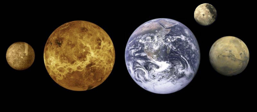
The silicate bodies of the Solar System (Mercury, Venus, Earth, the Moon and Mars). Image courtesy NASA/JPL-Caltech.
What exactly powers a planet?
In case of Earth 75% comes from radioactive element decay and the rest is the remnant heat (the trapped potential energy) from accretion times. Then, there’s another question: How old can a terrestrial planet be? According to BB theory, the universe is about 14 billion years old (well, 13.75 to be exact, but that is irrelevant here), and most elements are much younger. Even if galaxies appeared early in Universe history, I doubt there would be a habitable planet that old. Primordial gas giants? Perhaps, plenty. Primordial rocky objects? Not a chance.
After the Universe became more and more enriched in elements, the possibility for rocky planets to form eventually appeared. However, a planet, say, 7 billion years old (or older) would be powered by a different ratio of radioactive isotopes than an earth-aged planet. The age of chemical elements can be estimated using radioactive decay to determine how old a given mixture of atoms is.
The long-term thermal evolution of rocky planets depends on the abundance of the long-lived radioisotopes Th-232, U-235, and U-238 at the time of planet formation, and those are produced only during explosive nucleosynthesis (r-process) in stars with at least 8 to 20 solar masses (Chen et al. 2006).
Since we are talking about terrestrial planets, we are looking for silicates. In contrast to the abovementioned isotopes, silicon (Si) is produced by the whole range of massive stars. Thorium (Th) and uranium (U) are difficult to detect, but there is another element, europium (Eu), which is produced in the same reaction type (r-process) as Th and U, and can be measured. All r-process elements scale closely with solar values (Frebel 2008). This means that the average abundance of Th-232, U-235, and U-238 can be predicted from the europium trend with metallicity, the age-metallicity relationship and the star formation history of the Galaxy, and the half-life of each isotope. The average abundance of Eu to Si decreases by a factor of 0.63 as the metallicity increases by a factor of 100 to a solar value (Cescutti 2008).
An overwhelmingly large proportion of uranium on Earth is U-238. This makes it the heaviest atom commonly found in nature. U-238 and Th-232 have half-lives of 4.468 and 14.05 Gyrs respectively, but the uranium is underabundant in the Solar System compared to the expected production ratio in supernovae. This is not surprising since the U-238 has a shorter half-life.
Planets forming early in the history of the Galaxy would have 50% more U-238, but six times more U-235, than Earth. The higher abundance is because the amount of radioisotopes in the interstellar medium only reflects massive star formation over a few half-lives, whereas Si-28 and other stable isotopes accumulate over the history of the Galaxy. Therefore, these systems are silicon-poor. However, the high abundance of U-235 could have an important role in the early thermal history of such planets.
Heat transfer
Thermal energy from the hot interior of the planet flows out of the surface into space. When an object is at a different temperature than its surroundings, heat will transfer from the region of higher temperature to the region of colder temperature to achieve thermal equilibrium. The mantle transfers heat from the hot core at the planet’s center to the colder surface. When an upward heat flux passes through a fluid, the thermal energy is transported in two ways: conduction and convection. The control parameter that selects between the two regimes is the Rayleigh number.
In conduction the energy transfer occurs from hot vibrating atoms and molecules to neighboring atoms and molecules, while the fluid stays put, as if it were a solid. In a gravitational field, if temperature gradients in the mantle are large enough, instability due to buoyancy will cause convection.
Convection is heat transfer by the movement of fluid. The increase in temperature produces a reduction in density and the warm, buoyant material begins to rise, while colder, denser material near the surface is displaced and sinks. Convection transports heat more efficiently than conduction due to mass transport.
Mantles are predominantly solid rocky shells (getting more solid with depth), yet over very long time scales (tens to hundreds of millions of years) mantle rocks under extreme pressure and temperature slowly deform like a viscous fluid, moving in circular currents called convection cells.
Mantle convection ultimately drives all geological events, such as volcanoes, earthquakes, and plate tectonics. It moves continents to new positions. The continents, in turn, modify the flow inside the mantle due to “thermal blanketing”, acting like perfect thermal insulators. Thus, continental growth strongly affects mantle cooling.
Plate tectonics
Plate tectonics is a model in which the outer shell of a planet is broken into a number of thin rigid plates that move with respect to one another. The relative velocities of plates are of the order of a few tens of millimeters per year. Volcanism and tectonism are concentrated at plate boundaries. Much of Earth’s internal heat is relieved through this process and many of Earth’s large structural and topographic features are consequently formed.
Continental drift is cyclic and the main reason for this is the movement in convection cells. Ocean basins open and close, forming supercontinents, which later break apart again during another opening of the ocean; this process is known as the Wilson cycle.
Continental collision is one of the primary mechanisms for the creation of mountains in the continents; the other is subduction, the process when one tectonic plate moves under another, sinking into the mantle, as the plates converge. The Himalayas and the Alps are examples of mountain belts caused by continental collisions, and the Andes are associated with subduction. That’s the awesome power of Earth’s convection mode and gravity combined. In contrast, the extreme height of the Martian volcanoes can be attributed to the low surface gravity and the lack of relative motion between the lithosphere and the magma source.
During continental dispersal the sea level is high, and warm and humid maritime climate is dominant. The level of ocean floor spreading is high and relatively large amounts of carbon dioxide are produced at oceanic rifting zones. Seafloor spreading centers cycle seawater through hydrothermal vents, reducing the ratio of magnesium to calcium in the seawater through metamorphism of calcium-rich minerals in basalt to magnesium-rich clays (Wilkinson and Given, 1986; Lowenstein et al., 2001). This reduction in the Mg/Ca ratio favors the precipitation of calcite over aragonite, thus the seawater chemistry is that of a calcite sea.
During continental aggregation the ocean level drops due to lack of seafloor production. The cooler and arid continental climate dominates, corresponding with severe desert environments and frequent continental glaciations. The seawater chemistry is that of an aragonite sea, with high magnesium content.
The continental shelf has a very low slope and a small increase in sea level will result in a large change in the amount of flooded land. With averagely young world ocean the seafloor will be relatively shallow, making the sea level high with more landmass flooded. The old world ocean is relatively deep and more land will be exposed due to low sea level.
When continents are dispersed, the plate tectonic flux is high and Andean-type volcanism is extensive. With a single supercontinent and a low plate flux (the huge plate is a “blanket”) the mantle heats up due to the decay of radioactive isotopes. The increase in mantle temperature and the warming near the core–mantle boundary leads to an increase in the plume flux and the breakup of the supercontinent.
Implications to life
Continental spreads stimulate life diversity on evolutionary scale. Not only that, continental cycle influences the size of the species. According to Bergmann’s rule most mammals tend to be larger in cold climates and smaller in hot ones. The study by Smith et al.(2010) also shows that the colder the environment and the bigger the land surface, the bigger the large mammals become.
Tectonic environments and humans
Tectonic activity, as earthquakes and volcanoes, has a great influence on the course of development of civilizations and other complex cultures. Beside the obvious destruction, tectonism apparently accelerated cultural development. How this happened (and happens) exactly, is discussed in great detail in Tectonic Environments of Ancient Cultures blog by Eric Force.
A matter of mass
The mass of a planet is probably one of the most important properties regarding convection mode. Adding more mass can add troubles similar to that of reducing it (Venus, Mars). Earth might be a neat borderline case here, when things operate smoothly. Well, no one really knows for sure yet if plate tectonics will operate on massive planets, and regarding that there is a disagreement in the scientific community. Several studies were carried out and the results are quite interesting in all cases.
For my personal designs I have chosen a condition that plate tectonics does indeed operate on larger worlds (but not extremely large, though, because of several other factors). However, I take things from the other models into account as well.
There is also another thing worth mentioning here, a paper by Martyn Fogg (I have mentioned it in one of my previous posts). There, in section 3.2, page 7, is a formula (14) for estimating the duration of viable volcanic/tectonic recycling of volatiles on a given planet – basically, the timescale for plate tectonics. As the continent cycle goes on, increasing continental area would eventually initiate a transition between plate tectonics and a stagnant lid mode of mantle convection.
Plate tectonics is the primary mechanism through which Earth (and any planet with the same regime) loses its heat. Lenardic et al.(2005) suggests a potential constraint on continental surface area at which continental growth will stop. This critical point is predicted as a function of mantle heat flow. For the Earth’s current global heat flux, the critical continental surface area is estimated to be 35-50% to allow plate tectonics to initiate, and present day Earth’s continent crust area is about 40%.
So, how would things work on bigger planets?
There are several conditions necessary for plate tectonics to operate (Martin et al.,2008). First of all, the planet must have cooled enough so that it is too cold to sustain magma ocean. Second, its interiors must be hot enough to maintain convection within the upper layers of the body to prevent the existence of stagnant lid. Third, its lithosphere needs to be cool enough, strong enough, dense enough and thin enough to allow subduction. Fourth, liquid water on the surface is probably the most vital ingredient for successful plate tectonics.
Magnetic field lifetime is also tightly related to the thermal evolution of a planet. To drive dynamo action, a liquid metallic core must be in an active convection state.
Valencia et al. (2006), (2007) used planetary parameter scaling to argue that higher gravity favors subduction and plate tectonics are inevitable on larger terrestrial worlds. Nearly at the same time O’Neill and Lenardic (2007) proposed that super-sized Earths are likely to be in an episodic or stagnant lid regime.
As planet mass increases, it poses an increasingly severe problem for plate tectonics. Middle-aged super-Earths may suffer from continental spread, which could choke off plate tectonics, placing a planet in stagnant lid mode. Provided that crustal flow limits continental thickness, it was shown that continents will spread out to coat the surface of a terrestrial planet with more than three Earth masses in much less time than the age of the Earth (Kite et al., 2009).
More recent studies show that there might be another severe problem to plate tectonics on super-sized “Earths”. The convective pattern and the heat transport in a terrestrial planet depends on the viscosity of the mantle material. The viscosity, on the other hand, depends strongly on temperature and pressure, i.e., the viscosity decreases with increasing temperature but increases with increasing pressure. Thus, the larger the planet the stronger is the influence of the pressure on the viscosity and flowability of material. This dependence becomes an important factor for the mantle convection of planets with masses larger than one Earth mass. With more mass, planets are subject to sluggish convection regime in the lower mantle and formation of a conductive lid over the core-mantle boundary. Eventually convection stops and heat is transported only due conduction. Thermally induced magnetic field generation is suppressed as well. Compositional dynamos might also become suppressed due to small cooling rate of the inner core; such planets will end up with small surface magnetic fields, higher radiation environment and stronger atmospheric loss (Stamenkovic et al., 2010).
The results of another study using 2D spherical mantle convection model (Noack & Breuer, 2011) show that the propensity of plate tectonics has a peak at a specific mass: assuming viscosity increases with pressure, the peak occurs between one and five Earth masses. However, the variation of viscosity with pressure is strongly debated and might as well decrease with pressure (Karato, 2011, Icarus; Armann et al., 2010, Nature).
Tidally locked planets
This is another interesting case. If a planet lacks an atmosphere thick enough to balance the surface temperature, it will be in a stagnant lid convection regime at the night side and in a mobile regime at the day side. The reason for such difference is the upper convective mantle, which is sensitive to temperature variations on the surface (Noack et al., 2010).
The habitability of planets in synchronous rotation about their star may lie well outside the Habitable Zone (Gelman et.al 2011). Such world may still support liquid water on its surface, or shallow subsurface, in certain regions of the planet. Thus, tidally locked mantle and climate patterns must be combined and assessed to determine the surface environment, keeping in mind this may vary greatly from the substellar to antistellar regions.
# Well, this is it for now; maybe something will be added later.
This post is for those, who will be modeling their planet atmospheres in detail. If you have used Starform (accrete) code to generate your system and evolved the system with Mercury afterwards, using a climate model for your planet would be a good choice to continue.
Before I will go into details with data preparation and actual modeling, there are multiple issues with compiling some parts of the FORTRAN code, especially the ones containing f90 or fIV/f66 features. For *nix systems ifort and f90 compilers are the necessary choice.
Now, I know for sure f77, gfortran, g95 or FTN95 won’t be much help. (The latter is Windows only; now with this one I’m not exactly sure, but I couldn’t make it compile with 8 byte-integer AND real options, it allowed me one or another, and not both; even if it is possible, it is NOT OBVIOUS HOW at all.) For Windows users issues are resolved with Compaq Visual FORTRAN Professional v6.6, for example, or Intel’s ifort compiler if you have one. I like Compaq better because you don’t need to install Visual Studio additionally, and it handles pretty much everything. Please note that version 6.5 or lower won’t do because of the integer/real intrinsic data types support (8 bytes are necessary).
Once you are technically set, you can move onto the next phase of atmosphere/climate modeling – data preparation. It is also assumed that you have decided on the atmospheric composition. I’m not an astrophysicist, so everything I do below this point is what I have came up so far by guess, trial and error method (yes, I’m THAT persistent) and is not claimed to be flawless.
Comments, suggestions and corrections are welcome.
Data preparation
I’ll start with the 1-D coupled model and there are several things to do before actual modeling.
Stellar spectrum. If you are using BaSeL server, your output is the flux moment given in erg/cm^2/s/Hz/sr. To get this in ergs/s/cm^2/Hz you need to multiply it by PI to get rid of steradians (sr). Then, flux Flambda, in units ergs/s/cm^2/Angstrom, can be calculated using the equation Flambda=0.4*flux_moment*c/Lambda^2, where c=2.997925e17 is the velocity of light and Lambda is the wavelength in nanometers. The numerical factor of 0.4 (=4*0.1) in equation above comes from the conversion of the flux moment into flux (*4) and from the conversion of flux per nanometer into flux per Angstrom (*0.1). However Flambda still is a flux at the surface of a star.
The flux at the top of the atmosphere is used in models; the altitude of 100 km is taken as „the top”. For Earth, an altitude of 120 km marks the boundary where atmospheric effects become noticeable during spacecraft re-entry. Most of the atmosphere (99.9999 percent) is below 100 km, although in the rarefied region above this there are auroras and other atmospheric effects.
Now, flux, S, from a star drops off with increasing distance. In fact, it decreases with the square of the radial distance, r, from the star, as proportional to 1/r^2. You will need to provide distance in parsecs (see Stellar distance d in pc below).
Stellar flux with distance
There is also an option to obtain stellar spectrum by using ATLAS9 (or ATLAS12) and SYNTHE programs by Kurucz and Castelli (or SPECTRUM by Richard O. Gray, needs Atlas or MARCS stellar atmosphere model anyway). Here you can be more detailed with your star, providing additional initial conditions like microturbulent velocity* and mixing length parameter** into model. Then, there is also Chris Sneden’s MOOG.
*Microtubulent velocity. This is one of the fundamental stellar properties, a standard parameter in one-dimensional analyses of solar-type stars. For ATLAS models the value of microturbulent velocity, ξ, can be chosen [among 0, 1, 2, 4, etc. km/s] appropriate for the star’s surface gravity between the two velocities that bracket the microturbulent velocity. HOWEVER, the relation given by Kirby (Eq. 2 of Kirby et al. 2009, also here): ξ (km/s) = (2.13 ± 0.05) − (0.23 ± 0.03)*log g is only appropriate for giants, not sub-giants or dwarfs. Of course, for dwarfs there also exists a correlation between the luminosity class and the surface gravity (log g), the microturbulent velocity (t), and the metallicity ([M/H]) (Gray et al, 2000).
Dwarfs (V class) from F to G have the smallest microturbulent velocity, thus, technically, the higher the log g, the lower the microturbulent velocity. For precise results the technique of partial correlation can be employed, since the relationships between three or more random variables are being investigated. The trends for K stars (at least up to mid-K) are probably mainly similar to G dwarfs (Spectral studies of K dwarfs, Spectroscopic Properties of Cool Stars).
**Mixing length (ML) parameter. It is the alpha (a = l/Hp) parameter used in stellar model, which represents the ratio between the mean free path of a convective element (l) and the pressure scale height (Hp). The variations of this parameter strongly affect the structure of the outer envelope (i.e. radius and temperature). In fact, this parameter determines the efficiency of energy transport by convection in the outermost layer of a star: for a given stellar luminosity, it fixes the radius of the star, hence its temperature and color. In case of a real star, evolutionary tracks must then be calibrated by comparison with stellar radii and/or temperatures derived from observations. The most obvious ML calibrator is the Sun. The ML parameter can be fixed by constraining theoretical solar models (i.e. with solar mass, age and chemical composition) to reproduce the solar radius. In low-mass stellar models the derived stellar radii depend on the opacity which significantly contributes in determining the temperature gradient in their turbulent external layers. Hence, stellar models, based on different opacity tables, could require different values of alpha. It means that a homogeneous dataset of stellar temperatures at different metallicities to properly calibrate the ML parameter is urgently needed before any further attempt to use evolutionary models to derive relevant properties of stellar populations (Ferraro et al. 2006).
Lyman alpha flux at the planet (xLy). Lyman-alpha line is the brightest emission line of neutral hydrogen at the wavelength of 1215.67 A (121.567 nm) in the spectrum (in some papers 1215.7 A or 1216 A is mentioned). Stellar Lya emission lines are important spectral features in the context of exoplanet stellar environment and stellar physics. The Lya line is used as a proxy for determining the temperature and pressure profiles of upper stellar atmospheres. Lya flux is extremely variable with time. To a first approximation the solar La flux is composed of a quiet and of an active component. The Sun’s active component changes with the 27 days period (1 rotation around its axis); the quiet one with the 11 year solar cycle. For the Sun, the integrated Lya line flux may change by 37% during one rotation and up to 50% over a couple of years.
These fluxes can be obtained from the catalogue; in case of a synthetic star Lyman-alpha flux is the flux integrated over the whole Lya emission line of the synthetic spectrum. The easier way around is to compute a synthetic stellar Lya profile of a given linewidth, applying a simple linear rescaling in wavelength to the solar Lya profile. Real stellar profiles may be poorly represented by such a simple rescaling of the solar profile.
Math Box 1 – Some interesting data about your star
If you made yourself a synthetic star, some things are not given, but can be obtained through calculation. Now I was thinking if I need to include this in one of my posts, but heck, maybe it can be useful to someone.
If you know B-V color (from synthetic spectrum or from stellar data), then use it. Otherwise it can be calculated as B-V = (-3.684*LOG(Teff,K))+14.555. You can compare this data with the one from BaSeL result, for example, and make necessary adjustments.
Stellar rotation (vsin i)
Now, this one is tied to B-V and stellar age. I picked up formulas from (Barnes, 2007). Gyrochronology permits the derivation of ages for solar- and late-type main sequence stars using only their rotation periods and colors. If you know the age of your star and B-V color, you can go the other way around.
f(B-V) =0.7725*(((B-V)-0.4)^0.601), where B-V is the color;
g(t) = T^0.5119, where T is star age in Myr;
Rotational period P, days, is found as P = g(t)*f(B-V);
And finally, stellar equatorial rotational velocity, vsini, km/s, is found from the rotational period:
vsini = ((2*PI()*(R*2))/P)*(1/86400), where R is stellar radius and P is rotational period in days.
Stellar activity cycle
Approximate stellar cycle P, yrs, can be calculated as P = -1.22+(14.14*(B-V)). This is how long it takes your star to go from the minimum to maximum stellar activity. The complete cycle is, obviously, double of that.
Stellar distance d in pc. For your synthetic star you can take one of the provided distances (and manually scale the spectrum) for comparison with the VPL spectral data (I used 3.2 parsecs). If you used a real star, the real distance from Earth must be provided. It is needed for conversion to values expected for an Earth-like planet (see The Afac correction parameter). The flux will be scaled according to this distance.
The Afac correction parameter. To convert to values expected for an Earth-like planet, the measured UV fluxes were multiplied by ((206265*d )^2)*(Lsun/Lstar)*Afac, here d is the distance in parsecs (1 pc = 206264.806 =206205 AU), Lstar and Lsun are the respective bolometric luminosities of the star and the Sun, and Afac is a correction factor that accounts for the change in the planet’s albedo with the wavelength of the incident radiation. Values of Afac of 1.11 for the F2V star and 0.95 for the K2V star were obtained by scaling the “water loss” Seff limits in “Habitable Zones around Main Sequence Stars“, Kasting, J.F., Whitmire, D.P. & Reynolds, R.T. Icarus 101, 108-128 (1993), Table III, by the effective radiating temperature of the stars, using a quadratic fit to the listed temperatures. This procedure ensures that hypothetical planets would have the same surface temperature as the Earth (~288 K) if other climatic factors (e.g. cloudiness and greenhouse gas concentrations) are the same.
I went the other way around scaling given Afac numbers (x) to stellar temperatures (y):
x
y
notes
0.9
3450
(M3.5V, AD Leo)
0.95
5084
(K2V, ε Eridani)
1
5778
(G2V, Sun)
1.11
6930
(F2V, σ Boo)
Using quadratic regression I got coefficients for equation y=ax^2+bx+c:
a = -70906.1520; b = 158654.0223; c = -86698.5002
For any given temperature (K) within the range of [3450; 6930] you can solve the equation to find the roots:
Use the root that fits the range of Afac [0,9; 1,11] – in all cases here it will be x1.
Height of the tropopause. In planet.dat file you will need to provide the height of the tropopause. It is found to be strongly sensitive to the temperature at the planet’s surface through changes in the moisture distribution and its resulting radiative effects. The tropopause height is less sensitive to changes in the ozone distribution and hardly sensitive at all to moderate changes in the planet’s rotation rate (Thuburn & Craig, 1996).
Coupled photochemical and radiative/convective atmosphere model. When your data is ready, you can finally make executables and run your models. Make sure that everything in the files is set as you want it. And if you are running a coupled model, make sure your folder/file tree is put like it should be, and the couple switches in the code are on. Then, compile and run.
Some more alternatives
There is a very interesting model suite called Most for atmosphere and climate. It includes Planet Simulator, PUMA (The Portable University Model of the Atmosphere) and SAM (The Shallow Atmosphere Model) along with the Graphical User Interface, the Model Starter (MoSt), the postprocessor Burn7 and all manuals.
NOTE: There is no cake for Cygwin users here. You can get Most suite running under Cygwin (make sure X11 is properly set up), but the GUI is remarkably (read: awfully) slower than on Linux. Dual boot (Win/Linux) or “virtual machine” is the salvation.
# Have fun digesting and rejoice – there will be no more modeling for now (unless I’ll run into a proper planetary interior model. Yum.)
## Also, this is probably the last post this year but if you have questions or want to discuss something, feel free to drop a line. HAPPY WINTER HOLIDAYS and come back in January for more! 😉
This journal entry is dedicated to planetary atmospheres, since this is probably the most difficult part of a worldbuilder’s journey. Of course, you can have things easier way, say, if you have earthlike conditions or you have additional data laid out for you in case of a standard star. But what if things were different?
I’m going to explain each step, adding some theoretical info as well. The Four Elements series will cover topics such as the atmosphere, the ocean, geological activity, insolation and planetary climate. And maybe something else I’ll find necessary to add.
The quest doesn’t start where one might think it does – not on a planet, but on a star. So, long before we can model our planetary atmosphere or anything else related to it, first we should consider stellar spectrum. There are several ways of getting it: taking a real detailed spectrum for existing star or computing a synthetic stellar spectrum. It all depends on your star of choice and how deep you are willing to go into details.
Why is this important? To design your own exclusive and unique planetary atmosphere model: maybe the air is so thin at altitude of 5 km, so your local people will never go to the mountains, for example. Whatever it is, you’ll get the full set of necessary parameters, some of which you might have had imagined, and some of which you probably didn’t expect at all. Anyway, you will get to know your planet better.
Don’t be afraid of experimenting with things. They are not as hard or incomprehensible as might appear to be.
Planet atmosphere
The atmosphere is an envelope of gas mixture around the planet. It is held down by gravity, and the weight of that gas is pressure (as in mass times g). The total pressure is the sum of partial pressures of gasses in the mixture. The partial pressure is the contribution of a particular gas constituent to the total pressure, and is found as the total pressure times the volume fraction of gas component.
The proportion of gases found in the atmosphere changes with altitude. Distinct layers (such as troposphere, stratosphere, etc.) are identified using thermal characteristics, chemical composition, molecule movement, and density.
Individual molecules are moving freely in gas and if their motion velocity exceeds the planet’s escape velocity, the molecules will escape into space from the outer edge of the atmosphere. A certain amount will always exceed escape velocity, and if that percentage is too high, the atmosphere will leak away in a geologically short term. Thus, enough gravity is necessary to hold the atmosphere. The outer atmosphere temperature plays a vital role in this process as well, since gas molecules travel faster with increasing temperature. The hotter the exosphere is, the greater gravity must be. To keep things in balance, worlds closer to their stars must be larger to hold atmospheres equivalent to those around cooler worlds. Thus, atmospheric composition is also important, because lighter molecules move faster at the same temperature. Same surface gravity can keep one molecules, but can’t hold others; in case of Earth hydrogen and helium are too light for our gravity.
Composition and pressure are not completely free parameters, though. They are influenced and modified by chemical reactions with the surface of the planet (e.g. atmosphere interaction with crustal rocks over time in the carbonate-silicate cycle), living things and photodissociation (stellar UV light breaks up the hydrogen-bearing compounds like water, ammonia and methane) at the outer edge of the atmosphere. The atmosphere changes over geological time along with the evolution of the star, life and loss of lighter gasses.
Terrestrial-like planets may obtain atmospheres from three primary sources: capture of nebular gases, degassing during accretion, and degassing from subsequent tectonic activity. While capture of gases is vital for gas giants, low-mass terrestrial planets are unable to capture and retain nebula gases, which also may have largely dissipated from the inner solar system by the time of final planetary accretion. Atmospheric mass and composition for terrestrial planets is therefore closely related to the composition of the solid planet (Elkins-Tanton & Seager, 2008a).
In case of humans and animals the atmosphere has limits on its composition. To be breathable, it must have levels of molecular oxygen (O2) between 0.16 and 0.5 atm; higher concentrations of oxygen are toxic (severe cases can result in cell damage and death), lower than minimum are not enough to support human life. Hypoxia (oxygen deprivation) and sudden unconsciousness becomes a problem with an oxygen partial pressure of less than 0.16 atm. Hyperoxia (excess oxygen in body tissues), involving convulsions, becomes a problem when oxygen partial pressure is too high. Our present atmosphere contains 21% molecular oxygen (partial pressure of 0.21 atm).
Also, to prevent nitrogen narcosis under high pressures (the diver’s “rapture of the deep”) the partial pressure of nitrogen (N2) must be less than 3 atm.
As for other toxic stuff, the level of carbon dioxide must be less than 0.02 atm to breathe indefinitely, and less than 0.005 atm to avoid physiological stresses. In case of CO2 concentration above normal levels the only habitable places for humans might be high regions, like mountains. But then again, too little oxygen higher up can be troublesome.
Many plants, however, can survive and thrive in low oxygen-high CO2 environment. Earth’s plants will grow in many atmospheres that are unbreathable to humans and animals, unless the runaway greenhouse ruins the place completely (like Venus).
By building planet atmosphere and climate models you can see what are the boundaries for life under different stars and atmospheres. How fast the atmosphere thins upward? What are the properties of layers (altitudes, temperatures, pressures, composition, ozone layer (ozone is also toxic), gravitational pull, etc.)? What is the climate and weather pattern? The broader applications for the model include your planet aerospace or colonization/terraforming history, if applicable. The thickness of the atmosphere has some consequences. The thicker it is (and/or the lower the gravity), the easier flight is. Sound also travels better in a denser medium. Storms can be more intense if mass of moving air is greater.
More detailed description of atmospheres is beyond the scope of this article, but can be found on the Internet or in textbooks. In fact, if you know little about how atmospheres work, further reading into subject is required before building anything. Some useful book titles are listed in my LibraryThing catalogue, which is constantly growing. My goal here is to describe the tools: what data for models is required and how those models can be used to produce desirable results.
Climate dynamics model
The MITgcm (MIT General Circulation Model) is a numerical model designed for study of the atmosphere, ocean, and climate dynamics. MITgcm is freely available to all and can be run on a home pc or laptop, and is enough to play with your planet in detail.
Running the NASA/GISS model requires a significant investment in time and money, and it is designed to run on multiprocessor machines. It can reproduce the seasonal and regional mean values and variations of climate quantities such as temperature, pressure, precipitation, cloud cover, and radiation with reasonable degrees of precision, and many other things. I do not recommend this one for our purpose (though, if you own a multiprocessor workstation, you can try).
The CESM is also designed for simulating Earth’s climate system, but, as with the NASA/GISS, it is not simple at all. It is a coupled climate model composed of five separate models simultaneously simulating atmosphere, ocean, land, land-ice, and sea-ice.
However, before you can model weather and climate, an atmospheric layered model is required. You can take earthlike model (e.g. Standard Atmosphere) or you can make your own. For the latter purpose you’ll need another piece of code, described in the section below.
Photochemical and radiative/convective atmosphere models
This model requires stellar spectrum, which can be taken from the database or synthesized. Some spectra are hard to find. The ones used by Segura et al. can be taken from the VPL site.
Stellar flux greatly influences chemical processes in the atmosphere and biological processes on the planet. Each star has its individual flux “signature”.
In Segura’s model the “Earth” is assumed to be at a distance equivalent to 1 AU in the extrasolar planet system. The orbital radius is scaled according to stellar luminosity, and the planet is then moved inward or outward until its calculated surface temperature is 288 K. Also, the term “mixing ratio” has the same meaning as “mole fraction”.
Temperatures. Credit: Segura et al. 2003
The planet around the F star develops a thicker ozone layer because of the abundance of short-wavelength UV radiation (lambda < 200 nm) that can dissociate molecular oxygen.
Ozone number density. Credit: Segura et al. 2003
The surface UV flux increases with decreasing partial pressure of O2, but the behavior is very nonlinear. Good UV shield develops above 10^-2 of present atmospheric level of O2.
M stars emit very little near-UV radiation (200-300 nm), but active M (and, in fact, early K) stars emit lots of UV radiation shortward of 200 nm (chromospheric emission). One can therefore split molecular oxygen (and, hence, make ozone), but the ozone photochemistry is very different. Methane in Earth’s atmosphere is mostly destroyed in chemical reactions triggered by UV-flux at 310 nm. In atmospheres near M stars the lifetime for methane is long.
Synthetic stellar spectrum
If you have a star type that is not on the VPL list of spectra, acquiring a synthetic spectrum is where you’ll have to start building your model. There are numerous ways and software packages to compute a synthetic spectrum, but the easiest one is to use the BaSeL interactive server: it saves time and sanity. This tool presents a user-friendly interface of an interpolation engine, that allows on-line computations of synthetic stellar spectra for any given set of fundamental parameters Teff, log g and [Fe/H]. More info about BaSeL is found in “The BaSeL interactive web server: a tool for stellar physics”. Please note that fundamental parameters are taken from the real star’s data or computed stellar evolution model.