While procrastinating and enjoying my weekend I decided to go berserk on a full scale system building spree. This is the second part of the planetary system building series. The first part can be found here. I have updated it and made some corrections.
If you decided to make planets of your own after all, I suggest reading these papers: A Hybrid Symplectic Integrator that Permits Close Encounters between Massive Bodies, J. E. Chambers, 1998; Making More Terrestrial Planets, J. E. Chambers, 2001; Building the terrestrial planets: Constrained accretion in the inner Solar System, Raymond et al. 2009.
Now, let’s get down to our business.
In the previous post I promised to make a sample system. Here it is; you can use the following data as you like since I don’t plan to use it anywhere in my stories, but give me credit (or at least drop a comment here).
I have based my system on existing stars; this binary star system age estimations range from 6 to 8 Gyr (we’ll start somewhere at the beginning of the main sequence). The distance between the primary and the secondary is shortened to as close as 55 AU (the original distance is 1061 AU).
The primary has little or no variability and only low emission from its chromosphere.
Some notes on stellar evolution
You can build a system the same way I did; you can also use stellar model grids (as mentioned in this post, or the ones here and here, for example); or you can use this awesome Stellar Evolution Simulator to calculate parameters of your star’s evolution. You can also plot your personal H-R diagram after the simulation run.
When stars are studied spectroscopically it is found that most stars are composed of around 70% hydrogen and 28% helium by mass, very similar to what we see in the Sun. The fraction of all other elements is small and varies considerably from 2 or 3 % by mass in Sun-like stars (population I) to 0.1 to 0.01 percent by mass in stars found in globular clusters (population II). The Sun has about 1.8% heavy elements by mass.
Among the Solar-type stars observed in the Galaxy, many appear to be metal-rich relative to the Sun. The case of planets hosts is particularly interesting in that respect since they present, on average, an overmetallicity [Fe/H] of 0.2 dex. This metallicity is probably original, from the protostellar nebula, but it could also have been increased by accretion of hydrogen-poor material during the early stage of planetary formation.
Once nuclear fusion of hydrogen becomes the dominant energy production process and the excess energy gained from gravitational contraction has been lost, the star lies along a standard main sequence curve on the HR diagram. Astronomers will sometimes refer to this stage as “zero age main sequence”, or ZAMS. The ZAMS curve can be calculated using computer models of stellar properties at the point when stars begin hydrogen fusion. From this point, the brightness and surface temperature of stars typically increase with age.
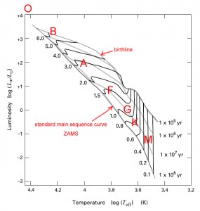
A star’s position on the ZAMS depends on both its mass and its initial helium abundance.
The mass fractions in H, He, and all elements heavier than He (“metals”) are labeled by the capitalized letters X, Y, and Z, respectively. They are related by: X + Y + Z = 1.
Often (Z/X) ratios are quoted, so
X = (1 + Y)/(1 + (Z/X))
Y = 1 – Z – Z/(Z/X)
Z = (1 – Y)/(1 + 1/(Z/X)).
Mazzitelli (1989) gives stellar evolution model with helium mass fraction depending on metallicity, in which helium content Y for stars is given by the empirical relation Y=0.243+(dY/dZ)*Z and where 0.243 is the primordial helium mass fraction. The reasonable value for dY/dZ is considered 2.0, though it is a very uncertain quantity and varies from object to object, e.g. the model with original solar values, Y = 0.267 and Z = 0.0188, would have a different dY/dZ value (note that X+Y+Z=1 must hold). An increase in Y decreases the main-sequence lifetime, and an increase in Z increases the main-sequence lifetime. The habitability for planetary systems is thus robust under changes in stellar model parameters (Jones et al. 2005).
Stars with higher initial helium abundances have higher luminosities and effective temperatures. This is predicted by homology; homologous stars are built with the assumption that star with mass M1 will just be a scaled version of a star with mass M0, because the physics which determines the structure of main sequence stars does not change rapidly with mass. Thus the higher mean molecular weight translates into lower core pressures. Helium rich stars therefore are more condensed, which mean they have higher core temperatures and larger nuclear reaction rates.
Changes in metallicity shift the location of the ZAMS; the metal-poor main sequence is blueward of the solar metallicity main sequence. This is primarily due to the reduced amount of bound-free absorption throughout the star (which only comes from metals). The smaller opacity of metal poor stars allows the energy to escape more easily, and thus increases the luminosity.
Typically the portion of heavy elements is measured in terms of the iron content of the stellar atmosphere, as iron is a common element and its absorption lines are relatively easy to measure. Because the molecular clouds where stars form are steadily enriched by heavier elements from supernovae explosions, a measurement of the chemical composition of a star can be used to infer its age.
My Primary is more enriched in heavy elements than the Sun, with almost two times solar abundance of iron; it is therefore classified as a rare “super metal-rich” (SMR) star. This abundance of metal makes estimating the star’s age and mass difficult, as evolutionary models are less well defined for such stars.
If you’re into stellar astrophysics, you might want to try and write your own code to simulate stellar structures and evolution. References: Stellar structure model, Stellar Modeling, The ATON 3.1 stellar evolutionary code and the ATON 3.1 stellar evolutionary code, a version for asteroseismology.
The model
Data Box 1 – Original stellar data
Star A, yellow dwarf, the primary
Spectral class: G8V
Mass: 0.95 solar masses
Radius: 1.152 solar radii
Luminosity (bolometric): 0.63 solar
Temperature: 5373 K
Apparent magnitude: 5.95
Absolute magnitude: 5.46
U−B color index : 0.65
B−V color index: 0.86
Metallicity: [Fe/H] = 0.31 (that makes Z = 0.038, greater than solar)Star B, red dwarf, the companion
Spectral class: M3.5-4V
Mass: 0.13 solar masses
Radius: 0.30 solar radii
Luminosity (bolometric): 0.0076 solar
Temperature: 3134 K (calculated)
Apparent magnitude: 13.15
Absolute magnitude: 12.66
U−B color index : 1.66
B−V color index: 1.21
Presumably the region this system formed in was dense and metal-rich. So I decided to go with six planets (and don’t forget the extra star). Three of them are terrestrials and the rest are gas and ice giants. Now, before you start arguing about various possible issues with this configuration, the plausibility of such system will be discussed in the upcoming Extension post, dedicated to binary and multiple star systems.
Data Box 2 – Planetary system data
Open/download all as text file.
Download archived files of the run and of the star evolution tracks.
The lifetime of the primary on the main sequence is about at least 11.37 Gyr (the greatest estimate was 14.6 Gyr). The companion star will have a very long life, at least twice that of the primary. So there is plenty of time to live.
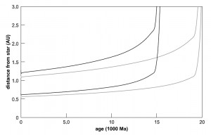
A brief calculation gave me current water & UV habitable zones for the primary between 0.8753 AU and 1.3574 AU, and the frost line at 2.436 AU. I have modeled probable evolution of the main star with Stellar Evolution Simulator and here is how the habzone might evolve.
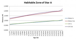
Planet E might (or eventually will) be habitable; I have no information on its atmosphere and leave it to your imagination. Even if it is truly ‘earthlike’, it will still be nothing like we know.
Planet F is the local “Jupiter”. It’s HUGE and it rotates faster than our Jupiter does. It probably has similar atmosphere, but with even more spectacular bands and local “giant spots”.
This is the chart of the system at the end of the final integration run.
Full system, front & side views:
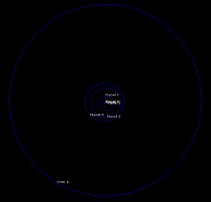

All planets, front & side views:
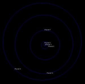
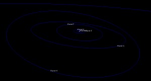
Four inner planets, front & side views:
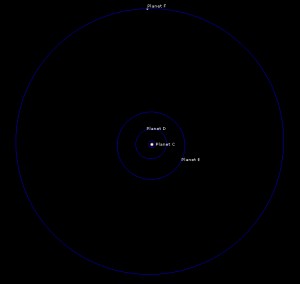
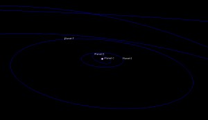
Terrestrial group, front & side views:
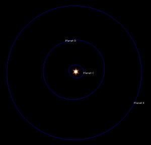

All ephemerids can serve as a good basis for you fictional calendar later. If you are a Celestia user, then you can easily make all these numbers into visually pretty 3D.
Noname system dynamics and stability
I did 100 000 year integration run to see if the system is stable at least that long. With the time step of 8 days for moderate accuracy it takes around 1 hour to do this on my spare machine (its CPU ticks at 789 MHz). One tenth of a million years is too little to see what’s really happening in this system and how it will evolve. Its components barely started to adjust to their would-be regular paths. Some of the orbits that might survive for 1-20 Myrs would very probably not survive for 1 Gyr.
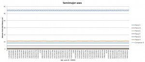
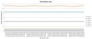
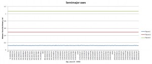
Here is a bunch of plots of orbital parameters from the final run (see initial data for it in Box 2).
Semimajor axes from full to detailed view:

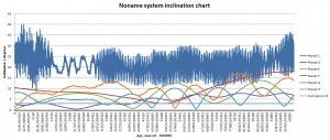
Inclinations of all major objects in the system:
Eccentricities of all system components:
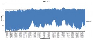
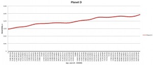
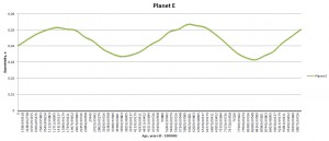
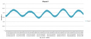
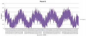
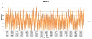
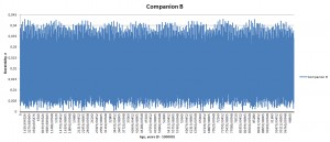
At first I have used inclination of 25 degrees, eccentricity of 0.055 and two different distances for star B. This had some strong effects on the planet C (closest to the primary): with companion B at a distance of 920 AU planet C was ejected into space somewhere at 54 000 years of integration; with companion B at a distance of 220 planet C became tilted at 100 degrees by the end of integration. The rest of the system remained relatively unaffected; e.g. the would-be habitable planet E didn’t have any scary shifts in eccentricity or obliquity (yet). Planetary rotation rates must be taken into account as well: they are less than 20 hours and this may give planetary axes additional stability. I didn’t include any moons into the system.
The “calm belt” is located between 0.4 and 5 AU as seen from orbital dynamics of planets D, E, and F. Planet F is the third massive body in the system after the primary and its companion. Planet C is strongly perturbed by star A; planets G and H are perturbed by both stars. If the system was real, the planets on G and H orbits may have never been formed.
Currently the system is widely chaotic; accidents might happen in the future. Planet C is probably the first candidate to fly away. Or maybe not.
What to watch for
1. Eccentricity (coupled with the distance from the primary)
Why? The orbital eccentricity of a habitable world might generally increase under the influence of other system bodies and might rise to the point where the planet is carried outside the HZ for a significant fraction of its orbital period. Whether a planet could be habitable in such a case depends on the response time of the atmosphere-ocean system; Williams & Pollard (2002) conclude that a planet like the Earth probably could.
2. Close encounters
The system bodies might perturb the orbit of the planet to the point it will be kicked out of the habitable orbital course or completely out of the system for good. Or even sent on a collision course with something not quite small (like a star or another planet; heck, even the moon will be enough). I don’t know what is worse in this case: being molten or frozen to death. In case of simply being kicked out of the system survival might still be possible with the help of technology, though.
3. Obliquity (axial tilt)
This is the most interesting part, since altogether with orbital parameters it governs insolation and climate of the planet. I will discuss this in detail in the appropriate post later on.
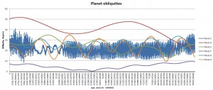
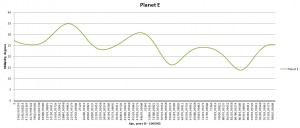
Here are the obliquities of planets in the noname system. The axial tilt of the earthlike world experiences quite large but not too severe variations (yet).
Obliquities:
Other experiments
Here is also an interesting simulation of the scenario when a planet inserted between the orbits of Mars and Jupiter. Multiple simulations were run, varying the eccentricity, orbital semi-major axis and mass of the inserted planet, and the resulting data analyzed with the help of visual data plots.

What utility are you using to generate your planetary stability plots?
The ones in the article are done in MS Excel, but I usually use gnuplot or MATLAB.