I’ve seen some debating on the Internet about Setting vs. Worldbuilding (here and here, for example). None of them provided a clear picture where the separation line should lie. But the separation line is so great, that, in fact, it is not just the line, it’s the whole damn canyon.
Setting exists only in a novel, play, film, etc. It has no purpose outside it. None. It is not the same as ‘worldbuilding’, because it is the immediate place and time of action, and the social environment of an individual, the POV character (and POVs are biased). It doesn’t go beyond that, but it sets the mood and it is what you currently see with your reader’s (viewer’s) eyes. Setting can be static or dynamic (depends on how the story is told), but it is not a process.
Worldbuilding, on the other hand, is the term describing a process of construction, engineering, if you must, of a fictional world regardless of how great/small it needs to be. It can include everything from physics to cultures, to languages and even music. It is a construction site of a ‘house’, in which each apartment can become a setting at some point in time. It’s a process of designing a framework, a ‘software package’ to write, debug, compile and build another piece of ‘software’ which is a story or what-have-you. You ‘build’ because you are structuring your ideas. You build a system. One of the great examples of such framework is the Orion’s Arm Project. It is self-sufficing and provides settings for stories. Another fine example are The Hard Return books by A. J. Klassen (AJ had published ‘book 0’ so far, but there are more on the way, and as a witness of the writing process and occasional consultant pal I can tell they’re awesome.) Love or hate it, but if you are a writer, a game designer, or anything of a sort, you are building a world.
Geofiction is almost self-explanatory. At least the ‘fiction’ part, which is exactly the statement of difference in purpose from worldbuilding. Geofiction includes everything worldbuilding does, but it exists for its own sake. A great example of geofiction is Planet Furaha.
Multiple star systems are not the majority in the Universe, even if in our Galaxy only 30 percent of stars are single, like our Sun. Massive stars tend to be more “family-oriented” than low-mass stars. For example, only 15 to 25 percent of M class stars are in binary or multiple systems comparing to 2/3 of G class stars, and G class makes only 7 percent of stars we see. The reason high-mass stars are often in multiples while low-mass ones are not is due to differences in how they form.
Star formation usually occurs in dense turbulent clouds of molecular Hydrogen. The natal environment influences star formation through the complex interplay of gravity, magnetic fields, and supersonic turbulence. Observations suggest that massive stars form through disk accretion in direct analogy to the formation of low-mass stars. However, several aspects distinguish high and low-mass star formation despite the broad similarity of the observed outflow and ejection phenomena.
Surprisingly, the nearby Taurus-Auriga star-forming region has a very high fraction of binaries for G stars and probably even for M stars. This produced a thought that most stars might be forming as multiples, but later these systems are broken apart.
High-mass vs. low-mass stars and the multiplet frequency
Low-mass star systems are observed to have a much lower binary fraction than higher mass stars (Lada 2006). In the recent simulations of a turbulent molecular cloud destined to form a small cluster of low-mass stars several classes of systems were produced: isolated stars, binaries and multiples formed via the fragmentation of a turbulent core, and binaries and multiples formed via the fragmentation of a disk; however, dynamical filament fragmentation is the dominant mechanism forming low-mass stars and binary systems, rather than disk fragmentation. (Offner et al. 2010). Loosely bound companions can be stripped by close encounters within the protocluster. Although previous studies suggested that multiple star formation via the fragmentation of a disk was limited to large mass ratio systems, recent work such as Stamatellos & Whitworth (2009) and Kratter et al. (2010a) has shown that when disks continue to be fed at their outer edges, the companions can grow substantially. Protostellar disks that are sufficiently massive and extended to fragment might be an important site for forming brown dwarfs and planetary mass objects (Stamatellos et al. 2011). Cores that form brown dwarfs would have to be very small and very dense to be bound (Offner et al. 2008).
Protostellar cores with a mass of a few tenths to a few hundreds of solar appear to be more turbulent, with gas within generally moving at higher velocities. Those are more prone to fragmentation, giving birth to binaries or multiple stars. Such massive star forming sites are rare and thus tend to be farther from Earth (> 400 pc) than low-mass star forming regions (around 100 pc). High-mass star formation occurs in clusters with high stellar densities. In addition, massive stars destroy their natal environment via HII regions. Their accretion disks are deeply embedded in dusty envelopes and ultra-compact HII regions become visible only after star formation is nearly complete. Observations of HII regions produced by massive stars are a prime tool for extragalactic astronomers to determine the star formation rate and abundances in galaxies.
Massive stars are shorter-lived and interact more energetically with their surrounding environment than their low-mass counterparts; they reach main sequence faster and begin nuclear burning while still embedded within and accreting from the circumstellar envelope. They also can be potential hazards to planetary formation: many low-mass stars are born in clusters containing massive stars whose UV radiation can destroy protoplanetary disks.
The temperature structure of the collapsing gas strongly affects the fragmentation of star-forming interstellar clouds and the resulting stellar initial mass function (IMF). Radiation feedback from embedded stars plays an important role in determining the IMF, since it can modify the outcome as the collapse proceeds (Krumholz et al. 2010). Radiation removes energy, allowing a collapsing cloud to maintain a nearly constant, low temperature as its density and gravitational binding energy rise by many orders of magnitude. Radiative transfer processes can be roughly broken into three categories: thermal feedback, in which collapsing gas and stars heat the gas and thereby change its pressure; force feedback, in which radiation exerts forces on the gas that alter its motion; and chemical feedback, in which radiation changes the chemical state of the gas (e.g. by ionizing it), and this chemical change affects the dynamics (Krumholz 2010).
Column densities L= 0.1, M=1.0, H=10.0 g cm-2 (left to right column). Credit: Krumholz et al. 2010
In this image surface column densities L= 0.1, M=1.0, H=10.0 g cm-2 are shown. As density increases, the suppression of fragmentation increases: (L) small cluster, no massive stars, depleted disks; (M) massive binary with 2 circumstellar disks and large circumbinary disk; (H) single large disk with single massive star.
The effects of radiative heating depend strongly on the surface density of the collapsing clouds, which determines effectiveness of trapping radiation and accretion luminosities of forming stars. Surface density is also an important factor in binary and multiple star formation. Higher surface density clouds have higher accretion rates and exhibit enhanced radiative heating feedback, diminished disk fragmentation and host more massive primary stars with less massive companions (Cunningham et al. 2011).
Observations indicate most massive O-stars have one or more companions; binaries are common (> 59%) (Gies 2008). Massive protostellar disks are unstable to fragmentation at R ≥ 150AU for a star mass of 4 or more solar masses (Kratter & Matzner 2006) and cores with masses above 20 solar will form a multiple through disk fragmentation (Kratter & Matzner 2007). Radiation pressure does not limit stellar masses, but the instabilities that allow accretion to continue lead to small multiple systems (Krumholz et al. 2009).
The upper limit on the final companion star frequency in the system can be estimated (Bate 2004).
Primordial stars and their legacy
The similar pattern appears in formation of previously believed to be solitary primordial stars. Recent studies suggest that loners were rather an exception, than the rule.
First massive stars were probably accompanied by smaller stars, more similar to our Sun. Due to encounters with their neighbors some of the small stars may have been ejected from their birth group before they had grown into massive stars. This could indicate primordial stars with a broad range of masses: short-lived, high mass stars capable of enriching the cosmic gas with the first heavy chemical elements and produced first black holes that are alive and well today, and long-lived, low-mass stars which could survive for billions of years and maybe even to the present day.
Are single stars really single?
Again, similar fragmentation happens in the massive protoplanetary discs to produce gas giants, when a gas patch in protoplanetary disk collapses directly into gas giant planet (1 Jupiter mass or larger) due to gravitational instability. Gravitational instabilities can occur in any region of a gas disk that becomes sufficiently cool or develops a high enough surface density, be it a star or a planet formation site. Kratter et al. 2009 suggests that planets formed that way might be failed binaries.
In 1970 Stephen Dole performed planet accretion simulation which produced interesting results. In our Galaxy, the average separation of binary components is about 20 AU, corresponding roughly to the orbital distances of the jupiter-mass gas giants in our solar system (Jupiter and Saturn have often been called “failed stars”; however, both probably contain rocky cores, so they are definitely planets). By increasing the density of the initial protocloud an order of magnitude higher than before, Dole’s program generated larger and larger jovians. Eventually in one high-density run, a class K6 orange dwarf star appears near Saturn’s present orbit, along with two superjupiters and a faint red dwarf further sunward. No terrestrials were formed.
Planetary system accretion. A is the density parameter. Solid circles – terrestrial planets, horizontal shading – gas giants, cross-hatching designate red dwarfs, open circle represents orange dwarf. Credit: S. Dole, 1970
This study suggested that Jovians (brown dwarfs can be mentioned here too now) multiply at the expense of terrestrials. An increase of one critical parameter – the nebular density – resulted in the generation of binary and multiple star systems, and close companionship might lead to eventual exclusion of terrestrial worlds.
But things appear to be more complicated.
Terrestrial planets in multiple star systems
Multiple star systems provide a complicated mix of conditions for planet formation, because the accretion potentially involves material around each star in addition to material around the group. These locations can provide opportunities as well as hazards.
Binary systems can have circumprimary (around the more massive star), circumsecondary (around the less massive star), and circumbinary (around both stars) disks, compared to likely routine planet formation sites around single stars. In widely spaced binaries you could even have protoplanetary discs around the two.
If there are no tidal effects, no perturbation from other forces, and no transfer of mass from one star to the other, a binary system is stable, and both stars will trace out an elliptical orbit around the center of mass of the system.
A multiple star system is more complex than a binary and may exhibit chaotic behavior. Many configurations of small groups of stars are found to be unstable, as eventually one star will approach another closely and be accelerated so much that it will escape from the system. This instability can be avoided if the system is hierarchical. In a hierarchical system, the stars in the system can be divided into two smaller groups, each of which traverses a larger orbit around the system’s center of mass. Each of these smaller groups must also be hierarchical, which means that they must be divided into smaller subgroups which themselves are hierarchical, and so on.
For a certain range of stellar separations, the presence of a companion star will clearly impact the formation, structure, and evolution of circumstellar disks and any potential planet formation. Global properties such as initial molecular cloud angular momentum, stellar density, the presence of ionizing sources and/or high mass, and so on, may all influence disk and thereby planet formation.
The maximum separation of bound systems is related to the stellar density. The denser clusters, in which most stars form, contain a lower fraction of bound multiple systems, comparable to the fraction found among field stars.
The binary star systems that host planets are very diverse in their properties and binary binary semimajor axes ranging from 20 AU to 6400 AU. In case where orbits are eccentric, the binary periastron can be as small as 12 AU, and important dynamical effects are expected to have occurred during and after planet formation.
In a circumbinary disk strong tidal interactions between the binary and disk are almost always expected, significantly affecting planet formation.
In a circumstellar disk with separations of a few to several tens of AU, the tidal torques of the companion star generate strong spiral shocks, and angular momentum is transferred to the binary orbit. This in turn leads to disk truncation, determining a “planet-free” zone (at least for formation). Subsequent dynamical evolution in multiple systems could still bring planets into this region.
For a circumstellar disk in a binary system, which is not influenced by strong tidal forcing, the effect of the companion star will be modest, unless the orbital inclinations are such that the Kozai effect becomes important.
Math Box 1 – The Truncation Radius
The truncation radius rt of the disk depends on the binary semimajor axis ab, its eccentricity eb, the mass ratio q = M2/M1 (M1, M2 denote the masses of the primary and secondary stars, respectively), and the viscosity v of the disk. For typical values of q = 0.5, eb = 0.3 and disk Reynold’s number of 10^5, the disk will be truncated to a radius of rt = 1/3ab.
For a given mass ratio q and semimajor axis ab an increase in eb will reduce the size of the disk while a large v will increase the disk’s radius. Not only will the disk be truncated, but the overall structure and density stratification may be modified by the binary companion.
In a circumbinary disk, the binary creates a tidally-induced inner cavity. For typical disk and binary parameters (e.g., eb = 0.3, q = 0.5) the size of the cavity is = 2.7 * ab.
Binary star diagram. Image courtesy of NASA
Numerical studies of the final stages of terrestrial planet formation in rather close binaries with separations of only 20–30 AU, that involve giant impacts between lunar-mass planetary embryos, show that terrestrial planet formation in such systems is possible, if there was a possibility for planetary embryos to form.
Systems with higher eccentricity or lower binary separation are more critical for planetesimal accretion. The effects of such eccentric companion include planetesimal breakage and fragmentation because of the increased relative velocities; the circumprimary planet forming disc truncation to smaller radii, causing the removal of material that may be used in the formation of terrestrial planets; destabilization of the regions where the building blocks for these objects may exist.
For binaries with separation less than 40 AU, only very low eccentricities allow planetesimal accretion to proceed as in the standard single-star case. On the contrary, only relatively high eccentricities (at least 0.2 in the closest 10AU separation and at least 0.7 for star system semimajor at 40AU) lead to a complete stop of planetesimal accretion.
A binary companion at 10 AU limits the number of terrestrial planets and the extent of the terrestrial planet region around one member of a binary star system.
Larger periastra (> 20AU) in solar-type binary star systems with terrestrial planets formation allow the stability of Jovian planets near 5 AU. These binary star/giant planets systems effectively support volatile delivery to the inner terrestrial region.
Approximately 40–50% of binaries are wide enough to support both the formation and the long-term stability of Earth-like planets in orbits around one of the stars. Approximately 10% of main sequence binaries are close enough to allow the formation and long-term stability of terrestrial planets in circumbinary orbits. According to this, a large number of systems can be habitable, given that the galaxy contains more than 100 billion star systems, and that roughly half remain viable for the formation and maintenance of Earth-like planets.
Math Box 2 – Stability of the satellite-type orbit, where the planet moves around one stellar component (S-Type Orbits).
In this equation, ac, the critical semimajor axis, is the upper limit of the semimajor axis of a stable S-type orbit, ab and eb are the semimajor axis and eccentricity of the binary, and mu = M2/(M1+M2). S-type orbits in binaries with larger secondary stars on high eccentricities are less stable. The +- signs define a lower and an upper value for the critical semimajor axis which correspond to a transitional region that consists of a mix of stable and unstable orbits.
Stability of the planet-type orbit, where the planet surrounds both stars in a distant orbit (P-Type Orbits).
For circular binaries, this distance is approximately twice the separation of the binary, and for eccentric binaries (with eccentricities up to 0.7) the stable region extends to four time the binary separation. A critical semimajor axis below which the orbit of the planet will be unstable is given by
Similar to S-type orbits, the +- signs define a lower and an upper value for the critical semimajor axis ac, and set a transitional region that consists of a mix of stable and unstable orbits.
Habitable zones in binary star systems
HZs in binaries depend the binaries’ orbital elements and the actual amount of radiation arriving at an orbiting planet. The analytical estimate on the extent of the HZs includes the radiation field of the binary as a function of spectral types, orbital parameters, as well as the relative orbital phase and calculations of the RMS (root-mean-square) and Min-Max distances of the inner and outer borders of the habzones in P-Type and S-Type configurations.
In a binary-planetary system, the presence of the giant planet enhances destabilizing effect of the secondary star. The Jovian planet perturbs the motion of embryos and strengthens their radial mixing and the rate of their collisions by transferring angular momentum from the secondary star to these objects.
Systems with close-in giant planets may require massive protoplanetary disks to ensure that while planetesimals and protoplanets are scattered as giant planets migrate, terrestrial bodies can form and be stable. Systems with multiple giants also present a great challenge to terrestrial planet formation since the orbital architectures of such systems may limit the regions of the stability of smaller objects.
Four different types of orbits are possible for a terrestrial planet in a binary system that hosts a Jovian planet: the terrestrial planet is inside the orbit of the giant planet; the terrestrial planet is outside the orbit of the giant planet; the terrestrial planet is a Trojan of the primary (or secondary) or the giant planet; the terrestrial planet is a satellite of the giant planet.
When numerically studying the dynamics of a terrestrial planet in a binary planetary system, integrations have to be carried out for a vast parameter-space. These parameters include the eccentricities, semimajor axes, and inclinations of the binary and the two planets, the mass-ratio of the binary, and the ratio of the mass of the giant planet to that of its host star. The angular variables of the orbits of the two planets also add to these parameters.
Except for a few special cases, the complexities of these systems do not allow analytical solutions of their dynamics, and require extensive numerical integrations. Those special cases are: binaries with semimajor axes larger then 100 AU in which the secondary star is so far away from the planet-hosting star that its perturbative effect can be neglected; binaries in which the giant planet has an orbit with a very small eccentricity (almost circular); binaries in which, compared to the masses of the other bodies, the mass of the terrestrial planet is negligible.
Instability is not the only hazard in multiple systems. The difference in masses and lifetimes can pose serious problems for life, especially in relatively close binaries or multiples.
Binary or multiple systems might be hosts to several generations of planets; life might arise and be wiped out several times in system’s lifetime. Here’s how such binary system might evolve: while both stars are on the main sequence and in close proximity to each other, small and close-in first generation of planets forms; eventually one star evolves from the main sequence into the red giant and the two stars spread further apart while stellar material blown off from the red giant builds a protoplanetary disk around the other star and second generation planets form; the second star eventually goes red giant giving the first star, which is now white dwarf, a protoplanetary disk which could create a third generation of planets.
Each generation of planets is built from stellar material with a sequentially increasing metallicity as the material is recycled within each star’s fusion processes. In this case it becomes possible for old stars, even those which formed as low metal binaries, to develop rocky planets later in their lifetimes.
However, not always changing environment might be a threat, like in case of this old gas giant PSR B1620-26 b.
Jovian planet in globular cluster M4. Credit: NASA
If such planet hosted habitable satellites, and host stars remained warm and safe enough to support life, inhabitants might not been affected much by dramatic changes. Or maybe they would. But that is another story.
# Pretty much everything in this article is presently under active research. To learn more about multiple star systems and habitable planets in them, try Planets in Binary Star Systems by Nader Haghighipour, 2010; or Multiple Stars across the H-R Diagram (you can read it online), 2005.
While procrastinating and enjoying my weekend I decided to go berserk on a full scale system building spree. This is the second part of the planetary system building series. The first part can be found here. I have updated it and made some corrections.
In the previous post I promised to make a sample system. Here it is; you can use the following data as you like since I don’t plan to use it anywhere in my stories, but give me credit (or at least drop a comment here).
I have based my system on existing stars; this binary star system age estimations range from 6 to 8 Gyr (we’ll start somewhere at the beginning of the main sequence). The distance between the primary and the secondary is shortened to as close as 55 AU (the original distance is 1061 AU).
The primary has little or no variability and only low emission from its chromosphere.
Some notes on stellar evolution
You can build a system the same way I did; you can also use stellar model grids (as mentioned in this post, or the ones here and here, for example); or you can use this awesome Stellar Evolution Simulator to calculate parameters of your star’s evolution. You can also plot your personal H-R diagram after the simulation run.
When stars are studied spectroscopically it is found that most stars are composed of around 70% hydrogen and 28% helium by mass, very similar to what we see in the Sun. The fraction of all other elements is small and varies considerably from 2 or 3 % by mass in Sun-like stars (population I) to 0.1 to 0.01 percent by mass in stars found in globular clusters (population II). The Sun has about 1.8% heavy elements by mass.
Among the Solar-type stars observed in the Galaxy, many appear to be metal-rich relative to the Sun. The case of planets hosts is particularly interesting in that respect since they present, on average, an overmetallicity [Fe/H] of 0.2 dex. This metallicity is probably original, from the protostellar nebula, but it could also have been increased by accretion of hydrogen-poor material during the early stage of planetary formation.
Once nuclear fusion of hydrogen becomes the dominant energy production process and the excess energy gained from gravitational contraction has been lost, the star lies along a standard main sequence curve on the HR diagram. Astronomers will sometimes refer to this stage as “zero age main sequence”, or ZAMS. The ZAMS curve can be calculated using computer models of stellar properties at the point when stars begin hydrogen fusion. From this point, the brightness and surface temperature of stars typically increase with age.
Pre-main sequence to ZAMS stellar evolution (masses 0.1 to 6 solar). Credit: The Formation of Stars. Steven W. Stahler and Francesco Palla, 2005
A star’s position on the ZAMS depends on both its mass and its initial helium abundance.
The mass fractions in H, He, and all elements heavier than He (“metals”) are labeled by the capitalized letters X, Y, and Z, respectively. They are related by: X + Y + Z = 1.
Often (Z/X) ratios are quoted, so
X = (1 + Y)/(1 + (Z/X))
Y = 1 – Z – Z/(Z/X)
Z = (1 – Y)/(1 + 1/(Z/X)).
Mazzitelli (1989) gives stellar evolution model with helium mass fraction depending on metallicity, in which helium content Y for stars is given by the empirical relation Y=0.243+(dY/dZ)*Z and where 0.243 is the primordial helium mass fraction. The reasonable value for dY/dZ is considered 2.0, though it is a very uncertain quantity and varies from object to object, e.g. the model with original solar values, Y = 0.267 and Z = 0.0188, would have a different dY/dZ value (note that X+Y+Z=1 must hold). An increase in Y decreases the main-sequence lifetime, and an increase in Z increases the main-sequence lifetime. The habitability for planetary systems is thus robust under changes in stellar model parameters (Jones et al. 2005).
HZs for a 0.9 solar mass star with the original values Y = 0.303, Z=0.0298 following the above-mentioned relation (black lines) and Y = 0.269 (solar value), Z = 0.0317 (increased metallicity) (grey lines). Credit: Jones et al, 2005.
Stars with higher initial helium abundances have higher luminosities and effective temperatures. This is predicted by homology; homologous stars are built with the assumption that star with mass M1 will just be a scaled version of a star with mass M0, because the physics which determines the structure of main sequence stars does not change rapidly with mass. Thus the higher mean molecular weight translates into lower core pressures. Helium rich stars therefore are more condensed, which mean they have higher core temperatures and larger nuclear reaction rates.
Changes in metallicity shift the location of the ZAMS; the metal-poor main sequence is blueward of the solar metallicity main sequence. This is primarily due to the reduced amount of bound-free absorption throughout the star (which only comes from metals). The smaller opacity of metal poor stars allows the energy to escape more easily, and thus increases the luminosity.
Typically the portion of heavy elements is measured in terms of the iron content of the stellar atmosphere, as iron is a common element and its absorption lines are relatively easy to measure. Because the molecular clouds where stars form are steadily enriched by heavier elements from supernovae explosions, a measurement of the chemical composition of a star can be used to infer its age.
My Primary is more enriched in heavy elements than the Sun, with almost two times solar abundance of iron; it is therefore classified as a rare “super metal-rich” (SMR) star. This abundance of metal makes estimating the star’s age and mass difficult, as evolutionary models are less well defined for such stars.
Star A, yellow dwarf, the primary
Spectral class: G8V
Mass: 0.95 solar masses
Radius: 1.152 solar radii
Luminosity (bolometric): 0.63 solar
Temperature: 5373 K
Apparent magnitude: 5.95
Absolute magnitude: 5.46
U−B color index : 0.65
B−V color index: 0.86
Metallicity: [Fe/H] = 0.31 (that makes Z = 0.038, greater than solar)
Star B, red dwarf, the companion
Spectral class: M3.5-4V
Mass: 0.13 solar masses
Radius: 0.30 solar radii
Luminosity (bolometric): 0.0076 solar Temperature: 3134 K (calculated)
Apparent magnitude: 13.15
Absolute magnitude: 12.66
U−B color index : 1.66
B−V color index: 1.21
Presumably the region this system formed in was dense and metal-rich. So I decided to go with six planets (and don’t forget the extra star). Three of them are terrestrials and the rest are gas and ice giants. Now, before you start arguing about various possible issues with this configuration, the plausibility of such system will be discussed in the upcoming Extension post, dedicated to binary and multiple star systems.
The lifetime of the primary on the main sequence is about at least 11.37 Gyr (the greatest estimate was 14.6 Gyr). The companion star will have a very long life, at least twice that of the primary. So there is plenty of time to live.
A brief calculation gave me current water & UV habitable zones for the primary between 0.8753 AU and 1.3574 AU, and the frost line at 2.436 AU. I have modeled probable evolution of the main star with Stellar Evolution Simulator and here is how the habzone might evolve.
Continuous HZ of star A
Planet E might (or eventually will) be habitable; I have no information on its atmosphere and leave it to your imagination. Even if it is truly ‘earthlike’, it will still be nothing like we know.
Planet F is the local “Jupiter”. It’s HUGE and it rotates faster than our Jupiter does. It probably has similar atmosphere, but with even more spectacular bands and local “giant spots”.
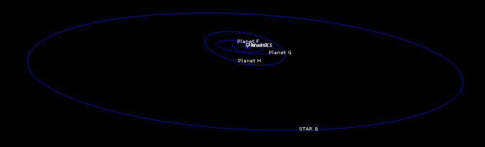
This is the chart of the system at the end of the final integration run.
Full system, front & side views:
Full system, head on viewAll planets, side view
All planets, front & side views:
Planet system, head-on viewAll planets, side view
Four inner planets, front & side views:
4 inner planets, head-on view4 inner planets, side view
Terrestrial group, front & side views:
Terrestrials, head-on viewTerrestrials, side view
All ephemerids can serve as a good basis for you fictional calendar later. If you are a Celestia user, then you can easily make all these numbers into visually pretty 3D.
Noname system dynamics and stability
I did 100 000 year integration run to see if the system is stable at least that long. With the time step of 8 days for moderate accuracy it takes around 1 hour to do this on my spare machine (its CPU ticks at 789 MHz). One tenth of a million years is too little to see what’s really happening in this system and how it will evolve. Its components barely started to adjust to their would-be regular paths. Some of the orbits that might survive for 1-20 Myrs would very probably not survive for 1 Gyr.
Here is a bunch of plots of orbital parameters from the final run (see initial data for it in Box 2).
Semimajor axes from full to detailed view:
Semimajor Axes, 0 – 100 000 yearsSemimajor Axes, 0 – 10 000 yearsSemimajor Axes closeup, 0 – 3000 yearsSemimajor Axes, Inner planets C, D and E. 0 — 3000 years
Inclinations of all major objects in the system:
Inclination i
Eccentricities of all system components:
Eccentricity of planet C, 0 – 100000 yearsEccentricity of planet D, 0 – 100000 yearsEccentricity of planet E, 0 – 100000 yearsEccentricity of planet F, 0 – 100000 yearsEccentricity of planet G, 0 – 100000 yearsEccentricity of planet H, 0 – 100000 yearsEccentricity of companion B, 0 – 100000 years
At first I have used inclination of 25 degrees, eccentricity of 0.055 and two different distances for star B. This had some strong effects on the planet C (closest to the primary): with companion B at a distance of 920 AU planet C was ejected into space somewhere at 54 000 years of integration; with companion B at a distance of 220 planet C became tilted at 100 degrees by the end of integration. The rest of the system remained relatively unaffected; e.g. the would-be habitable planet E didn’t have any scary shifts in eccentricity or obliquity (yet). Planetary rotation rates must be taken into account as well: they are less than 20 hours and this may give planetary axes additional stability. I didn’t include any moons into the system.
The “calm belt” is located between 0.4 and 5 AU as seen from orbital dynamics of planets D, E, and F. Planet F is the third massive body in the system after the primary and its companion. Planet C is strongly perturbed by star A; planets G and H are perturbed by both stars. If the system was real, the planets on G and H orbits may have never been formed.
Currently the system is widely chaotic; accidents might happen in the future. Planet C is probably the first candidate to fly away. Or maybe not.
What to watch for
1. Eccentricity (coupled with the distance from the primary)
Why? The orbital eccentricity of a habitable world might generally increase under the influence of other system bodies and might rise to the point where the planet is carried outside the HZ for a significant fraction of its orbital period. Whether a planet could be habitable in such a case depends on the response time of the atmosphere-ocean system; Williams & Pollard (2002) conclude that a planet like the Earth probably could.
2. Close encounters
The system bodies might perturb the orbit of the planet to the point it will be kicked out of the habitable orbital course or completely out of the system for good. Or even sent on a collision course with something not quite small (like a star or another planet; heck, even the moon will be enough). I don’t know what is worse in this case: being molten or frozen to death. In case of simply being kicked out of the system survival might still be possible with the help of technology, though.
3. Obliquity (axial tilt)
This is the most interesting part, since altogether with orbital parameters it governs insolation and climate of the planet. I will discuss this in detail in the appropriate post later on.
Here are the obliquities of planets in the noname system. The axial tilt of the earthlike world experiences quite large but not too severe variations (yet).
Obliquities:
Obliquities, 0 – 100 000 yearsObliquity of planet E, 0 – 100 000 years
Other experiments
Here is also an interesting simulation of the scenario when a planet inserted between the orbits of Mars and Jupiter. Multiple simulations were run, varying the eccentricity, orbital semi-major axis and mass of the inserted planet, and the resulting data analyzed with the help of visual data plots.
This month’s post is long and quite complex. So I will split it in two parts: Input & Output. I also decided to write an Extension post to the series, where I will discuss binary and multiple star systems, and things related.
Designing an extremely realistic planet (along with the whole system) is not a simple task, so if you have no interest in it, I suggest you don’t read math & tech parts of this article (I will mark them as such). We’ll be doing some math here and there. Also, advanced level of computer knowledge is required. If you don’t know what a command line is, skip those parts and enjoy the rest. And last but not least, this task will require a few days of your time (mostly computer time though). So, if you have something to do, like mow grass on the football field, now is a perfect opportunity. With all this said I’m moving onto the main thing.
Countless planetary systems exist throughout the vastness of space. Some of them are small, consisting only of one planet per star; some of them are big, like our Solar System with 8 planets and lots of other stuff orbiting around the Sun. In fact, all planetary systems discovered up until now consist of smaller number of planets than the Solar System, with 2 to 4 planets being most common.
Before designing your own system it might be a good idea to look through descriptions of those systems. There are numerous catalogues with data. For example:
For more planet stuff you can also read the Systemic blog, which is written by Greg Laughlin, Professor of Astronomy and Astrophysics at the University of California, Santa Cruz. Systemic reports recent developments in the field of extrasolar planets, with a particular focus on observational and theoretical astronomical research work supported by the NASA Astrobiology Institute, and by the Foundational Questions Institute (FQXi).
Now, there are two ways of getting your system up: top-to-bottom or bottom-to-top methods.
The top-to-bottom method suggests using some of the accretion algorithms to generate your system – you’ll get all stuff automatically, nothing to invent there. And I’m not talking about “planetary system generators” found on the web (e.g. StarGen), they don’t produce realistic systems. They tend to produce systems “similar to our own”; the truth is planetary systems don’t follow this “similarity” plan. A truly alien world will be something else, as you can see from worlds discovered up to date. Personally, at some point I’ve been using AstroSynthesis (v.3.0 will be released somewhere after September 30th). It does cool things, try it. I recommend it to those who don’t want to go deep into calculations.
State-of-the-art planetary accretion simulations typically use N-body integrations, but these are too computationally expensive and time consuming. So we’ll skip that part and get to the time when all planets are already in their respectful places. Trust your intuition; it’s better than some generator.
The bottom-to-top method implies you first imagine your main planet and do all the necessary calculations for its parameters (I will talk about those in detail below). The rest of the system is rather sketchy: all you decide is where to put other planets (semimajor axes) and how many there will be in total (you can also add some of their details as well, e.g. mass, density and orbital elements). This decision should be based on your star of choice and its parameters.
Planetary parameters
I assume you have already decided on mass, density and calculated radius. If not, check the previous post here.
Another two parameters required for our computations are axial tilt and rotation rate. The tilt can be anything you want from 0 to 180°. Note that object with tilt below 90° has a retrograde rotation, like Venus does. Also, planets usually move on their orbits in counterclockwise direction, with clockwise direction being retrograde orbital motion.
There are three cases of planetary rotation around its axis: normal (counterclockwise), retrograde and tidally locked (synchronous rotation or orbital resonance, e.g. Mercury’s 3:2 spin-orbit resonance).
When planets are born, they have their primordial spins. During their lifetimes planetary spins are affected by solar tides and tides inflicted by another bodies of the system. Planets and moons slow down, spin up (like Mars and Saturn did), or become tidally locked if too close to a star or any other massive body (e.g. Mercury, the Moon). Earth’s initial spin rate was about 6.5 hours comparing to modern 24 hour day.
Math Box 1 – Initial rotation of a planet
Approximate initial planetary spin can be estimated from its mass.
First, you calculate initial angular velocity using Dole’s equation (output is in rad/s). M is the mass of the planet; k is the moment of inertia ratio (I/MR^2), a value of 0.33 is taken for a terrestrial planet (you can look at planet moments of inertia in these fact sheets); r is planet’s radius, and j is 1.46E-20 m²/s²kg.
ω = [(2*j*M) / (k*r^2)] ^ 0.5
Then, initial rotation rate in seconds is calculated as t = (2*PI)/ω
Now, from this point onward things start to slow down, because a tidal deceleration torque from the primary is applied. (On some occasions things might actually spin up.)
Here (dωe/dt) = (-1.3E-6 /10^9) rad s-1/yrs; k is as mentioned above for terrestrials; m is a planetary mass; index letter e stands for Earth and p for planet.
You can estimate planetary angular velocity at any age of the system. In the following formula system age is in seconds. The new angular velocity then becomes
ωnew = Initial angular velocity ω + (system age (s) * tidal deceleration torque dω/dt)
Rotation rate in seconds is calculated >> t = (2*PI)/ωnew
In hours >> th = t/3600
Thus you can determine how your planet day becomes longer. However, the primary isn’t the only one influencing rotation rate of a planet. There’s also atmospheric drag, and a small influence of the system’s bodies. (Some of the formulas above are taken from Fogg, 1992.)
Note: If you have a moon or two, things get more complicated. You’ll have to take them into account as well.
Note 2: I suggest you calculate rotation rate this way instead of integrating the whole system for considerable amount of time; that could take days on an average machine, especially if precision and long timespan (more than 100×10^8 to X × 10^9 years) are chosen.
Angular velocity also gives us a clue to planetary flattening and difference between polar and equatorial radii.
Math Box 3 – Planet flattening (dynamical ellipticity) and radii
The radius you determined from mass and density is the mean radius, R. If not, the time is now:
R=0.5*[(mass/density)*(6/PI)]^(1/3)
or, if given mass and log g, through relation
Mstar/Msun=((Rstar/Rsun)^2)*10^(loggstar-loggsun).
Ellipticity e = SQRT(f*(2-f)) is related to flattening, which can then be expressed as f = 1-SQRT(1-e^2) or f = (1/SQRT(1-e^2))-1; or, if you have only radii, flattening becomes f=(Re-Rp)/R.
Flattening f is also calculated as f* = (5/4)*(((ω^2)*(R^3))/(M*G)); ω – from calculations above (math box 1 & 2); R – mean radius; M – planetary mass; G = 6.67259E-11. Equatorial radius thus becomes Re = R*(1+(f/3)), and polar Rp = R*(1-((2*f)/3)). The difference between radii is expressed as Re-Rp, or simply as mean R*f.
*Note: We’ll get somewhat overestimated degree of rotational flattening of the planet because the formula takes planet’s interior as incompressible fluid of uniform density. In reality terrestrial planet’s core is much denser than its crust. Or, in case of gaseous planets, an overestimate will rise from the fact that they have a mass distribution which is strongly concentrated at their cores.
Now, when we have our rotation rates, we can move onto the next step.
Orbits and orbital elements
The traditional orbital elements are the Keplerian elements. They describe the orbit of the body in space.
Keplerian elements can be obtained from and converted to orbital state vectors (x-y-z coordinates for position and velocity) by manual transformations or with computer software. For our integration Keplerian elements should be enough. If you want something else, the body-centered, inertial rectangular components of the radius vector can be determined from the classical orbital elements (see math box 4).
Math Box 4 – Orbital State Vectors
The mean longitude λ = M + ω + Ω where M is the mean anomaly, ω is the argument of perigee, Ωis the longitude of the ascending node.
The true anomaly ν is found from the expression ν=λ-Ω-ω
The body-centered, inertial rectangular components of the radius vector can be determined from the classical orbital elements as follows:
Position formulasVelocity formulas
Here a is the semimajor axis, e is the eccentricity, i is the inclination; in these equations p is called the semiparameter of the orbit and is calculated from p=a*(1-e^2). η is the gravitational constant of the primary or central body.
Math Box 5 – The spin angular momentum*
*this will be necessary for the main integration part to calculate obliquities and spin rates. If you won’t do integration, skip this part.
SAM is a vector, it has 3 components. It is calculated as H = H * Ĥ
H = 0.4 * M * (R^2) * v
Here, R is planet’s equatorial radius, M is planetary mass, and v is a spin rate (angular velocity).
The initial coordinates of unit vector Ĥ in the reference frame are:
X = sin ψ * sin ε
Y = cos ψ * sin ε
Z = cos ε
Where ψ is precession in longitude and ε is axial tilt of a planet.
The precession in longitude ψ is defined by ψ = L – Ω, where Ω is the longitude of the ascending node, and L is the inclination of ecliptic. The angle between the planet’s equatorial plane and inclination of ecliptic is the obliquity ε.
Your both precession angle ψ and obliquity ε should be in radians.
**You can calculate your precession rate as well. Note that precession formulas use semimajor axis (a) and eccentricity (e). You can start integration at the beginning of the system age (if you have time and patience) to get all things neatly; or you can skip to the necessary age and use the “invented” data as initial point. Whatever works for you.
The final step is to multiply each component of Ĥ by the quantity H.
Hx = H * X
Hy = H * Y
Hz = H * Z
Integration will require these quantities in AU^2/day, so take mass as Mass/Mass of the star, R of a planet as R/149597870.7, and angular velocity in radians/day.
TECH TOOLBOX: Environment and Integrator
Note: Numerous programs exist to perform integrations of n-body systems. If you want to learn more, google something like “n-body integrator”.
Mercury is written in Fortran77 in a slightly non-standard code and before you can use it, you have to compile it. So, first of all, you need a compiler. I used GNU gfortran for this purpose. Depending on your operating system there are some options:
Assuming you installed all necessary things, we now can move onto our main goal – Mercury package.
The package has the manual, the file called mercury6.man and can be opened with any text editor of your choice. Read it CAREFULLY and follow all the instructions.
If using gfortran, compile the drivers typing lines
gfortran -o mercury6 mercury6_2.for
gfortran -o element6 element6.for
gfortran -o close6 close6.for
To run what you have compiled, just type
./mercury6
and hit enter.
Pretty simple.
If you have questions regarding installation and usage, feel free to ask. But please note that I’m running all this under Windows XP and might not know about any issues with other operating systems.
So far I had no issues with any software mentioned here.
Integration of orbits
When integrating the equations of motion in classical or relativistic celestial mechanics, one has to know the values of the parameters, in particular the masses and the initial conditions (orbital parameters or state vectors). I won’t be going into the n-body problem details here. If you are interested I suggest reading some good literature on the subject, e.g. Gravitational N-body Simulations: Tools and Algorithms by Sverre J. Aarseth (a cheap copy can be found on abebooks.com or on any of their international sites).
So far all necessary info on required parameters is in the Mercury manual.
Are planetary systems stable? Probably. You can’t tell just by looking at them; the invisible force out there guides all the interactions between the bodies. That’s why scientists perform numerical integrations of planetary orbits.
#For the next part I’ll do a small sample system integration.